2  Distributions

library("ggplot2"); theme_set(theme_bw())

2.1 Discrete

2.1.1 Bernoulli

2.1.2 Binomial

2.1.3 Poisson

2.1.4 Negative binomial

2.2 Continuous

2.2.1 Normal

2.2.2 Logistic

We say a random variable \(X\) has a logistic distribution if it has the following probability density function. \[f(x) = \frac{e^{-(x-\mu)/\sigma}}{\sigma\left(1 + e^{-(x-\mu)/\sigma} \right)^2}\] with

• location parameter \(\mu\),
• scale parameter \(\sigma > 0\), and
• \(-\infty < x < \infty\).

We write \(X \sim Lo(\mu,\sigma)\) and \(E[X] = \mu\) and \(Var[X] = \sigma^2 \pi^2 / 3\).

As can be seen in the plot below, the logistic distribution has much heavier tails than the normal distribution.

# Compare logistic and normal pdfs (same mean/variance)
ggplot(data.frame(x = c(-3, 3)),
       aes(x = x)) +
  stat_function(fun = dlogis, args = list(scale = 3 / pi^2)) + 
  stat_function(fun = dnorm, color = "red", linetype = "dotted")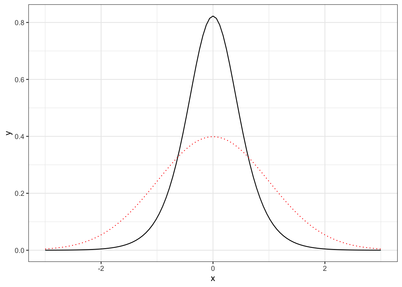 

The logistic distribution gets is name from its cumulative distribution function which is a member of the logistic functions.

\[F(x) = \frac{1}{1 + e^{-(x-\mu)/\sigma}}\]

The logistic distribution can be utilized in a latent variable representation of logistic regression.