Previously, we calculated the margin of victory (home score minus away score) and constructed a model for the margin of victory. In those models, we estimated a team strength and used the difference in team strengths to calculate the expected margin of victory and game outcome probabilities.
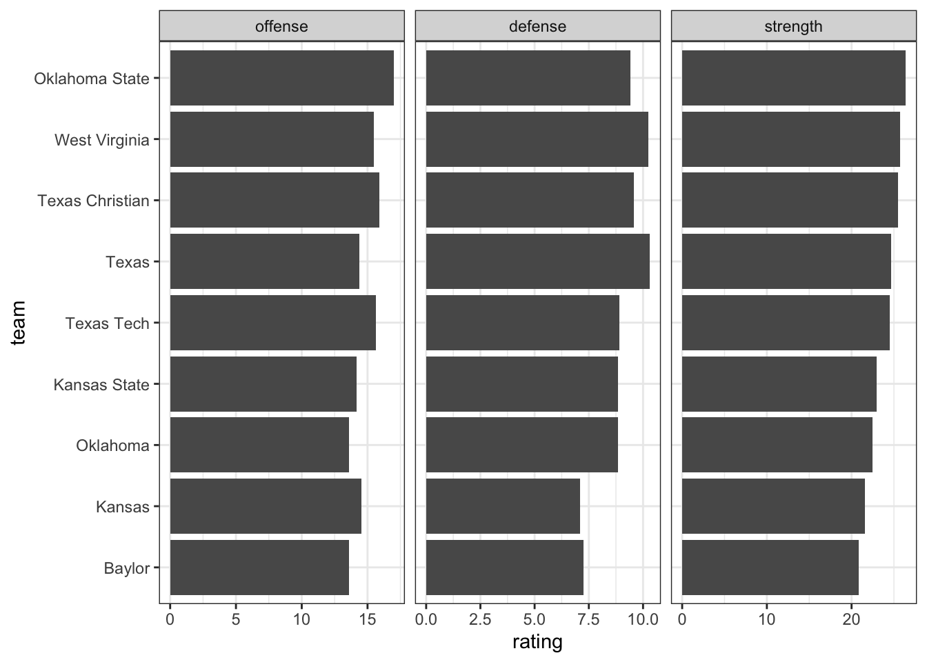
In this chapter, we will build models for the both the home score and the away score. Using the scores allows us to estimate offense and defense team strengths.
9.1 Model
A model for the number of points scored by the home team is
This error arises because if two teams play each other repeatedly we would expect the home score would be random around the expected home score.
The parameters are
\(\eta\) is the offensive home advantage,
\(\theta_t\) is the offensive strength of team \(t\), and
\(\delta_t\) is the defense strength of team \(t\).
The expected home score when team \(H\) is at home playing against team \(A\) is
\[E\left[S^H\right] = \eta + \theta_{H} - \delta_{A}.\] We can build a similar model for the away team score. A model for the number of points scored by the away team is
This error arises because if two teams play each other repeatedly we would expect the away score would be random around the expected away score.
The expected away score when team \(H\) is at home playing against team \(A\) is
\[E\left[S^A\right] = \theta_{A} - \delta_{H}.\]
We can utilize these models to calculate the expected margin of victory \(M\) for home team \(H\) playing away team \(A\): \[\begin{array}{rl}
E[M]
&= E[S^H - S^A] \\
&= E[S^H] - E[S^A] \\
&= \eta + \theta_H - \delta_A - (\theta_A - \delta_H) \\
&= \eta + (\theta_H + \delta_H) - (\theta_A + \delta_A)
\end{array}
\] where
\(\eta\) is the home advantage,
\(\theta_H - \delta_H\) is the strength of the home team, and
\(\theta_A - \delta_A\) is the strength of the away team.
9.1.1 Identifiability
In this model, when two teams play each other, the score is expected to be the home advantage \(\eta\) plus the difference in strengths between the two teams \(\theta - \delta\). Thus, only the difference between the offense and defense rating is identifiable. and we can arbitrarily add a constant to all of the \(\theta\) and \(\delta\) values.
9.1.2 Regression
If we assume \(\epsilon_g^H, \epsilon_g^A \stackrel{ind}{\sim} N(0,\sigma^2)\), then this is a linear regression model.
Since we have both the offensive parameters (\(\theta\)s) and defensive parameters (\(\delta\)s), we will need to construct a home matrix \(X^H\) and an away matrix \(X^A\).
For \(X^H\) we have \[X^H_{g,t} = \left\{
\begin{array}{rl}
1 & \mbox{if team $t$ is the {\bf home} team in game $g$} \\
0 & \mbox{otherwise}
\end{array} \right.\]
For \(X^A\) we have \[X^A_{g,t} = \left\{
\begin{array}{rl}
1 & \mbox{if team $t$ is the {\bf away} team in game $g$} \\
0 & \mbox{otherwise}
\end{array} \right.\]
Compared to the model matrices we created earlier, we have no negative values (-1) in these matrices.
Let \(S^H\) (\(S^A\)) be the score for the home (away) team in an upcoming game. The regression model assumes \[
S^H \sim N(\eta + \theta_H - \delta_A, \sigma^2)
\quad \mbox{and (independently)} \quad
S^A \sim N(\theta_A - \delta_H, \sigma^2).
\] Thus, the margin of victory \(M\) is \[
M = S^H - S^A \sim N(E[M], 2\sigma^2)
\] where \[E[M] = \eta + (\theta_H + \delta_H) - (\theta_A + \delta_A).\]
To find the probability the home team wins we use \[P(M > 0)
= P\left( T_v > \frac{-E[M]}{\sigma\sqrt{2}} \right)
= P\left( T_v < \frac{ E[M]}{\sigma\sqrt{2}} \right)
\] where \(T_v\) is a T-distribution with \(v\) is the degrees of freedom. The degrees of freedom can be calculated using \(v = 2(G-T)\).
If \(G >> T\) (which is certainly not true in our simple example), then \(T_v \stackrel{d}{\approx} Z\) (where \(\stackrel{d}{\approx}\) means approximately equal in distribution). Thus, we can calculate the probability using \[
P(M > 0) \approx P\left( Z < \frac{ E[M]}{\sigma\sqrt{2}} \right).
\]
The standard deviation here is
(sd <-summary(m)$sigma)
[1] 7.920613
Suppose Team 1 plays against Team 2 at Team 1’s home.
# Margin of Victory: Team 1 (Home) - Team 2 (Away)expected_margin <-as.numeric(coef(m)[1] + teams[1, "strength"] - teams[2, "strength"]) # Probability of Victory: Team 1 (Home) - Team 2 (Away)pt(expected_margin / (sd *sqrt(2)), df =summary(m)$df[2])
[1] 0.9052297
9.2 Examples
9.2.1 2023 Intraconference Big12 Baseball
# Big 12 2023 Intraconference games# I'm not sure why the file uses 2024baseball <-read.csv("../../data/college_baseball_2024.csv") |># Create home/away teams and scores# for neutral sites, home/away will be arbitrarymutate(Home_Field =gsub("@", "", Home_Field),home_is_Team_1 =# this is used repeatedly below Home_Field =="neutral"| Home_Field == Team_1, # Set the teamshome =ifelse(home_is_Team_1, Team_1, Team_2),away =ifelse(home_is_Team_1, Team_2, Team_1),# Set the scoreshome_score =ifelse(home_is_Team_1, Score_1, Score_2),away_score =ifelse(home_is_Team_1, Score_2, Score_1),Date =as.Date(Dates, format ="%m/%d/%Y") ) |>filter(Home_Field !="neutral") |>select(Date, Home_Field, home, away, home_score, away_score)
      Date             Home_Field            home               away
 Min.   :2023-03-17   Length:109         Length:109         Length:109
 1st Qu.:2023-04-01   Class :character   Class :character   Class :character
 Median :2023-04-16   Mode  :character   Mode  :character   Mode  :character
 Mean   :2023-04-17
 3rd Qu.:2023-05-01
 Max.   :2023-05-20
   home_score       away_score
 Min.   : 0.000   Min.   : 0.000
 1st Qu.: 4.000   1st Qu.: 3.000
 Median : 7.000   Median : 6.000
 Mean   : 7.394   Mean   : 5.963
 3rd Qu.:10.000   3rd Qu.: 8.000
 Max.   :20.000   Max.   :21.000