3 Regression

library("tidyverse"); theme_set(theme_bw())

── Attaching core tidyverse packages ──────────────────────── tidyverse 2.0.0 ──
✔ dplyr     1.1.4.9000     ✔ readr     2.1.5     
✔ forcats   1.0.0          ✔ stringr   1.5.1     
✔ ggplot2   3.5.1          ✔ tibble    3.2.1     
✔ lubridate 1.9.3          ✔ tidyr     1.3.1     
✔ purrr     1.0.2          
── Conflicts ────────────────────────────────────────── tidyverse_conflicts() ──
✖ dplyr::filter() masks stats::filter()
✖ dplyr::lag()    masks stats::lag()
ℹ Use the conflicted package (<http://conflicted.r-lib.org/>) to force all conflicts to become errors

library("ggResidpanel")

3.1 Simple Linear Regression

3.1.1 Model

For observation $i = \{1,2,\ldots,n\}$, let

$Y_i$ be the response variable and
$X_i$ be the explanatory variable.

The simple linear regression model (SLR) assumes \[ Y_i \stackrel{ind}{\sim} N(\beta_0 + \beta_1 X_i, \sigma^2) \] or, equivalently, \[ Y_i = \beta_0 + \beta_1 X_i + \epsilon_i, \quad \epsilon_i \stackrel{ind}{\sim} N(0, \sigma^2). \]

3.1.2 Interpretation

Recall \[ E[Y_i] = \beta_0 + \beta_1 X_i \]

Thus,

$\beta_0$ is the expected response when $X_i=0$
$\beta_1$ is the expected increase in the response when $X_i$ is increased by 1.

3.1.3 Assumptions

Recall \[ E[Y_i] = \beta_0 + \beta_1 X_i, \quad \epsilon_i \stackrel{ind}{\sim} N(0, \sigma^2) \]

Thus, the model assumptions are

The errors are independent.
The errors are normally distributed.
The errors have constant variance.
The relationship between the expected response and the explanatory variable is a straight line.

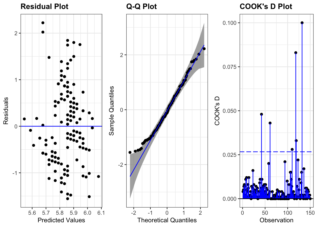
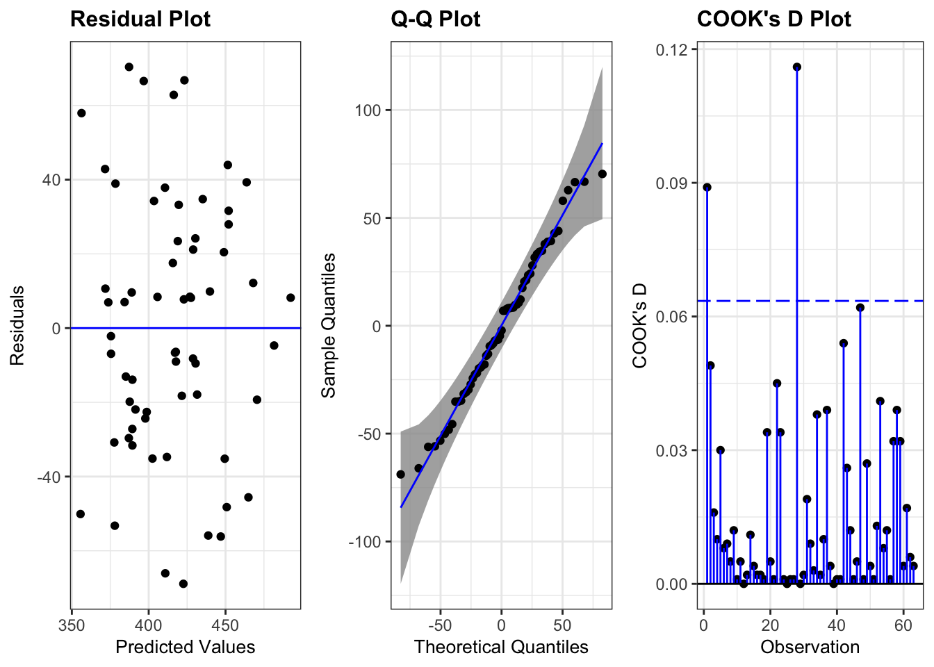
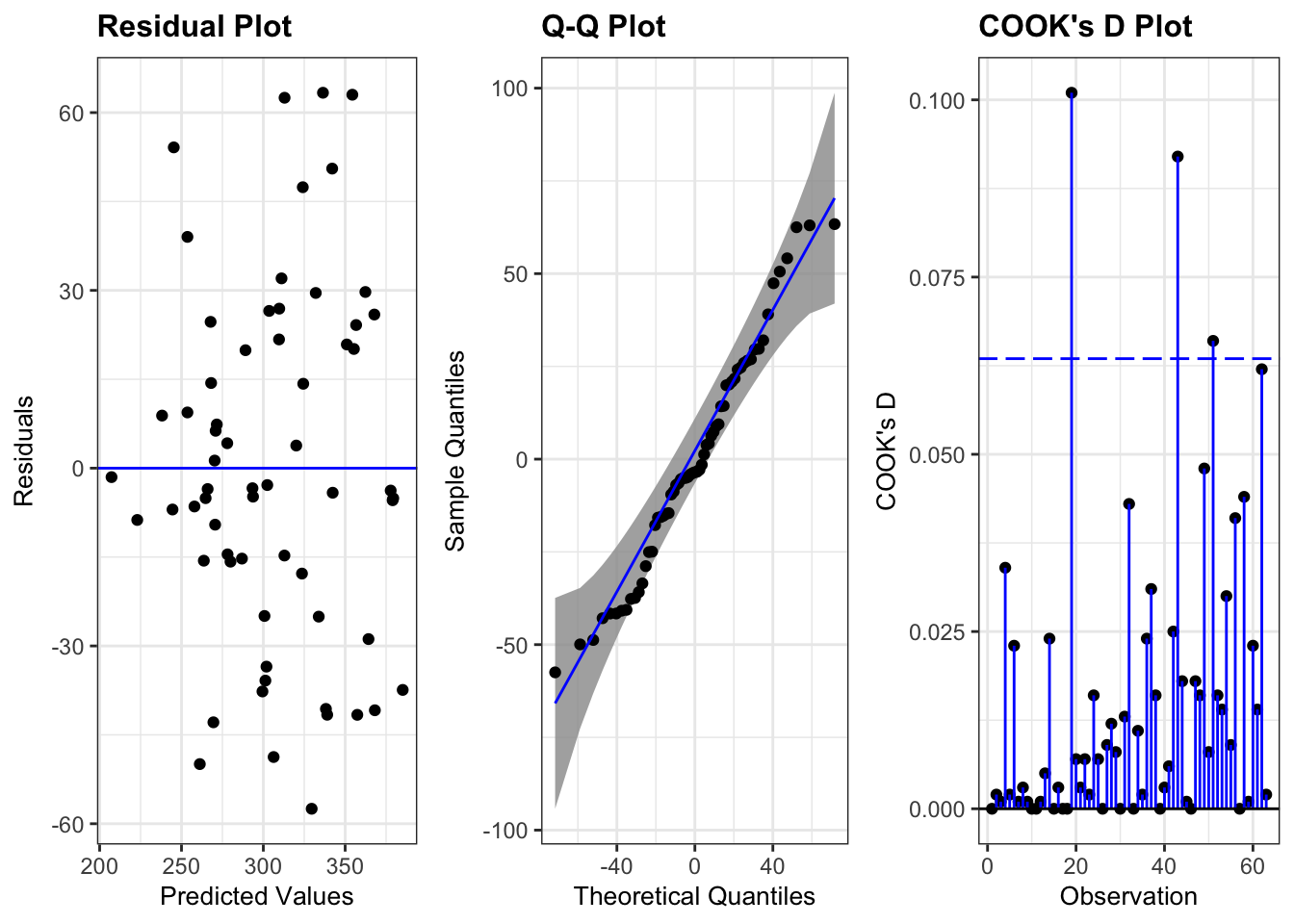
3.1.4 Diagnostics

m <- lm(Sepal.Length ~ Sepal.Width, data = iris)
ggResidpanel::resid_panel(m, 
                          plots = c("resid", "qq", "cookd"), 
                          qqbands = TRUE, 
                          nrow = 1)

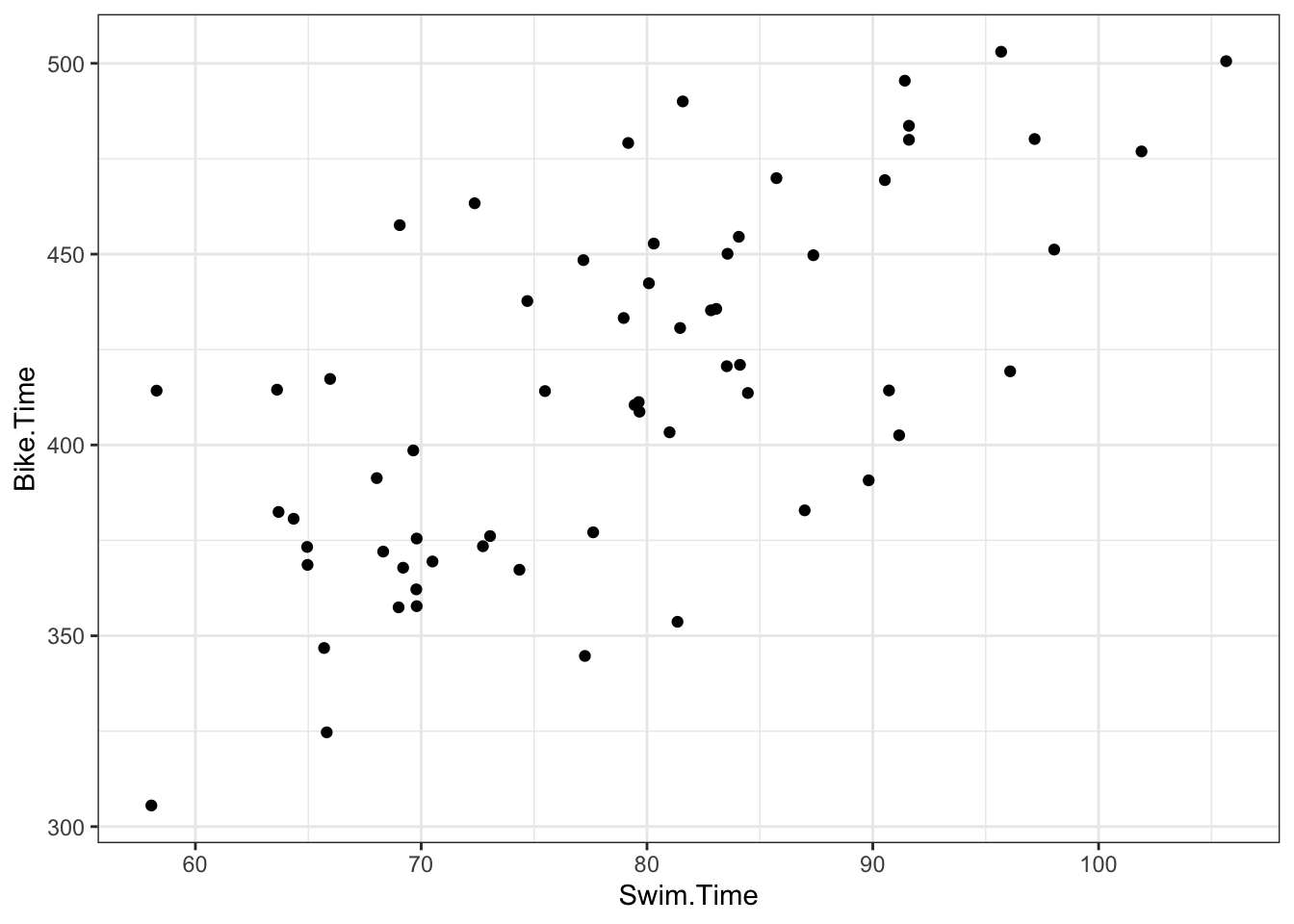
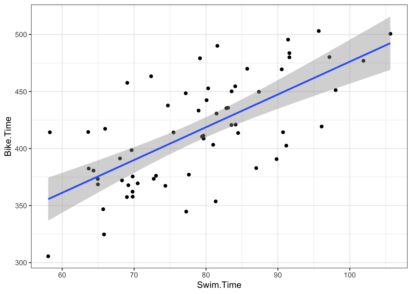
3.1.5 Triathlon Data

d <- read_csv("data/ironman_lake_placid_female_2022_canadian.csv")

Rows: 64 Columns: 17
── Column specification ────────────────────────────────────────────────────────
Delimiter: ","
chr  (6): Name, Country, Gender, Division, Finish.Status, Location
dbl (11): Bib, Division.Rank, Overall.Time, Overall.Rank, Swim.Time, Swim.Ra...

ℹ Use `spec()` to retrieve the full column specification for this data.
ℹ Specify the column types or set `show_col_types = FALSE` to quiet this message.

head(d)

# A tibble: 6 × 17
    Bib Name     Country Gender Division Division.Rank Overall.Time Overall.Rank
  <dbl> <chr>    <chr>   <chr>  <chr>            <dbl>        <dbl>        <dbl>
1     2 Melanie… Canada  Female FPRO                 5         575.           21
2     9 Pamela-… Canada  Female FPRO                10         610.           51
3  1000 Carley … Canada  Female F35-39               4         660.          126
4  1935 Seanna … Canada  Female F45-49               3         665.          131
5   511 Marie-C… Canada  Female F45-49               4         679.          161
6  1240 Julie H… Canada  Female F40-44               6         693.          202
# ℹ 9 more variables: Swim.Time <dbl>, Swim.Rank <dbl>, Bike.Time <dbl>,
#   Bike.Rank <dbl>, Run.Time <dbl>, Run.Rank <dbl>, Finish.Status <chr>,
#   Location <chr>, Year <dbl>

ggplot(d |> filter(Swim.Time < 500), 
       aes(x = Swim.Time, y = Bike.Time)) + 
  geom_point()

m <- lm(Bike.Time ~ Swim.Time, data = d |> filter(Swim.Time < 500))
ggResidpanel::resid_panel(m, plots = c("resid", "qq", "cookd"), qqbands = TRUE, nrow = 1)

summary(m)


Call:
lm(formula = Bike.Time ~ Swim.Time, data = filter(d, Swim.Time < 
    500))

Residuals:
    Min      1Q  Median      3Q     Max 
-68.901 -23.468  -2.169  23.808  70.369 

Coefficients:
            Estimate Std. Error t value Pr(>|t|)    
(Intercept) 188.8604    32.0893   5.885 1.82e-07 ***
Swim.Time     2.8729     0.4035   7.120 1.44e-09 ***
---
Signif. codes:  0 '***' 0.001 '**' 0.01 '*' 0.05 '.' 0.1 ' ' 1

Residual standard error: 34.83 on 61 degrees of freedom
Multiple R-squared:  0.4538,    Adjusted R-squared:  0.4449 
F-statistic: 50.69 on 1 and 61 DF,  p-value: 1.443e-09

cbind(coef(m), confint(m))

                            2.5 %     97.5 %
(Intercept) 188.860386 124.693942 253.026829
Swim.Time     2.872855   2.065987   3.679724

summary(m)$r.squared

[1] 0.4538433

When swim time is 0, the expected Bike Time is 189 mins with a 95% interval of (125, 253). For additional minute of swim time, the bike time is expected to increase 2.9 mins
(2.1, 3.7). The model explains 45% of the variability in bike time.

ggplot(d |> filter(Swim.Time < 500), 
       aes(x = Swim.Time, y = Bike.Time)) + 
  geom_point() + geom_smooth(method = "lm")

`geom_smooth()` using formula = 'y ~ x'

3.1.6 Two-sample T-test

We can use SLR to compare two groups.

Note that \[ Y_i \stackrel{ind}{\sim} N(\mu_{g[i]}, \sigma^2) \] where $g[i] \in \{1,2\}$ determines the group membership for observation $i$

is equivalent to \[ Y_i \stackrel{ind}{\sim} N(\beta_0 + \beta_1 \mathrm{I}(g[i] = 2), \sigma^2) \] where $\mathrm{I}(g[i] = 2)$ is the indicator function, i.e. \[ I(A) = \left\{ \begin{array}{ll} 1 & A\mbox{ is TRUE} \\ 0 & \mbox{otherwise} \end{array} \right. \] % i.e. $I(A) = 1$ if $A$ is true and $I(A) = 0$ otherwise,

and \[ \mu_1 = \beta_0 \quad \mbox{and} \quad \mu_2 = \beta_0 + \beta_1. \]

d2 <- d |> filter(Division %in% c("F40-44", "F45-49"))

d2 |>
  group_by(Division) |>
  summarize(
    n = n(),
    mean = mean(Bike.Time),
    sd = sd(Bike.Time)
  )

# A tibble: 2 × 4
  Division     n  mean    sd
  <chr>    <int> <dbl> <dbl>
1 F40-44      13  435.  43.6
2 F45-49      18  405.  39.5

ggplot(d2, aes(x = Division, y = Bike.Time)) + 
  geom_boxplot(outliers = FALSE, color = "gray") + geom_jitter(width = 0.1)

m <- lm(Bike.Time ~ Division, data = d2)
summary(m)


Call:
lm(formula = Bike.Time ~ Division, data = d2)

Residuals:
    Min      1Q  Median      3Q     Max 
-61.663 -32.237   3.556  27.806  95.406 

Coefficients:
               Estimate Std. Error t value Pr(>|t|)    
(Intercept)      435.13      11.44  38.040   <2e-16 ***
DivisionF45-49   -29.97      15.01  -1.996   0.0554 .  
---
Signif. codes:  0 '***' 0.001 '**' 0.01 '*' 0.05 '.' 0.1 ' ' 1

Residual standard error: 41.24 on 29 degrees of freedom
Multiple R-squared:  0.1208,    Adjusted R-squared:  0.09051 
F-statistic: 3.986 on 1 and 29 DF,  p-value: 0.05535

Comparison to two-sample t-test:

cbind(coef(m), confint(m)) # Regression results

                            2.5 %      97.5 %
(Intercept)    435.1295 411.73435 458.5246236
DivisionF45-49 -29.9693 -60.67155   0.7329461

t.test(Bike.Time ~ Division, 
       data = d2, 
       var.equal = TRUE) # Two-sample t-test


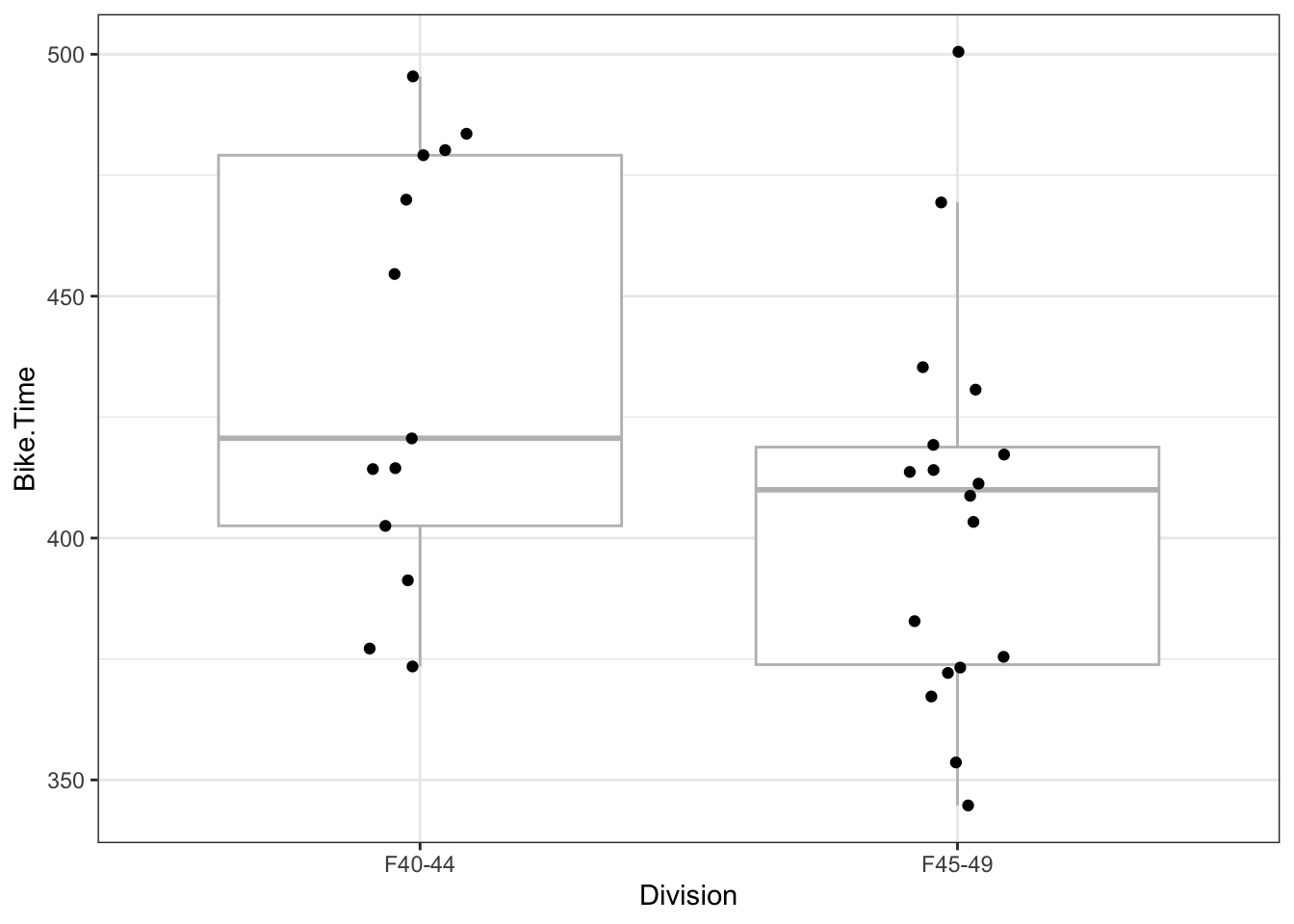
    Two Sample t-test

data:  Bike.Time by Division
t = 1.9964, df = 29, p-value = 0.05535
alternative hypothesis: true difference in means between group F40-44 and group F45-49 is not equal to 0
95 percent confidence interval:
 -0.7329461 60.6715501
sample estimates:
mean in group F40-44 mean in group F45-49 
            435.1295             405.1602

3.2 Multiple Linear Regression

3.2.1 Model

For observation $i = \{1,2,\ldots,n \}$, let

$Y_i$ be the value of the response variable and
$X_{i,j}$ be value of the $j$th explanatory variable

The (multiple linear) regression model assumes \[ Y_i = \beta_0 + \beta_1 X_{i,1} + \beta_2 X_{i,2} + \cdots + \beta_p X_{i,p} + \epsilon_i \]

and \[ \epsilon_i \stackrel{ind}{\sim} N(0, \sigma^2). \]

3.2.2 Interpretation

Recall \[ E[Y_i] = \beta_0 + \beta_1 X_{i,1} + \beta_2 X_{i,2} + \cdots + \beta_p X_{i,p} \]

Thus,

$\beta_0$ is the expected response when all $X_{i,j} = 0$
$\beta_j$ is the expected increase in the response when $X_{i,j}$ is increased by 1 and all other explanatory variables are held constant

When multiple regression is used, you will often see people write the phrases after controlling for'' orafter adjusting for’’ followed by a list of the other explanatory variables in the model.

3.2.3 Assumptions

Recall \[ E[Y_i] = \beta_0 + \beta_1 X_{i,1} + \beta_2 X_{i,2} + \cdots + \beta_p X_{i,p}, \quad \epsilon_i \stackrel{ind}{\sim} N(0, \sigma^2) \]

Thus, the model assumptions are

The errors are independent.
The errors are normally distributed.
The errors have constant variance.
The relationship between the expected response and the explanatory variables is given above.

3.2.4 Diagnostics

m <- lm(Run.Time ~ Swim.Time + Bike.Time, data = d |> filter(Swim.Time < 500))
ggResidpanel::resid_panel(m, plots = c("resid", "qq", "cookd"), 
                          qqbands = TRUE, nrow = 1)

ggResidpanel::resid_xpanel(m)

3.2.5 Example

ggplot(d |> filter(Swim.Time < 500),
       aes(x = Swim.Time, y = Run.Time, color = Bike.Time)) +
  geom_point()

ggplot(d |> filter(Swim.Time < 500),
       aes(x = Bike.Time, y = Run.Time, color = Swim.Time)) +
  geom_point()

summary(m)


Call:
lm(formula = Run.Time ~ Swim.Time + Bike.Time, data = filter(d, 
    Swim.Time < 500))

Residuals:
    Min      1Q  Median      3Q     Max 
-57.474 -16.782  -3.523  21.298  63.349 

Coefficients:
            Estimate Std. Error t value Pr(>|t|)    
(Intercept) -68.0058    35.1258  -1.936   0.0576 .  
Swim.Time    -0.3771     0.4773  -0.790   0.4326    
Bike.Time     0.9726     0.1119   8.689  3.3e-12 ***
---
Signif. codes:  0 '***' 0.001 '**' 0.01 '*' 0.05 '.' 0.1 ' ' 1

Residual standard error: 30.45 on 60 degrees of freedom
Multiple R-squared:  0.6711,    Adjusted R-squared:  0.6602 
F-statistic: 61.22 on 2 and 60 DF,  p-value: 3.238e-15

Written summary

cbind(coef(m), confint(m))

                              2.5 %   97.5 %
(Intercept) -68.0057881 -138.267938 2.256362
Swim.Time    -0.3771479   -1.331933 0.577637
Bike.Time     0.9725912    0.748696 1.196486

summary(m)$r.squared

[1] 0.6711405

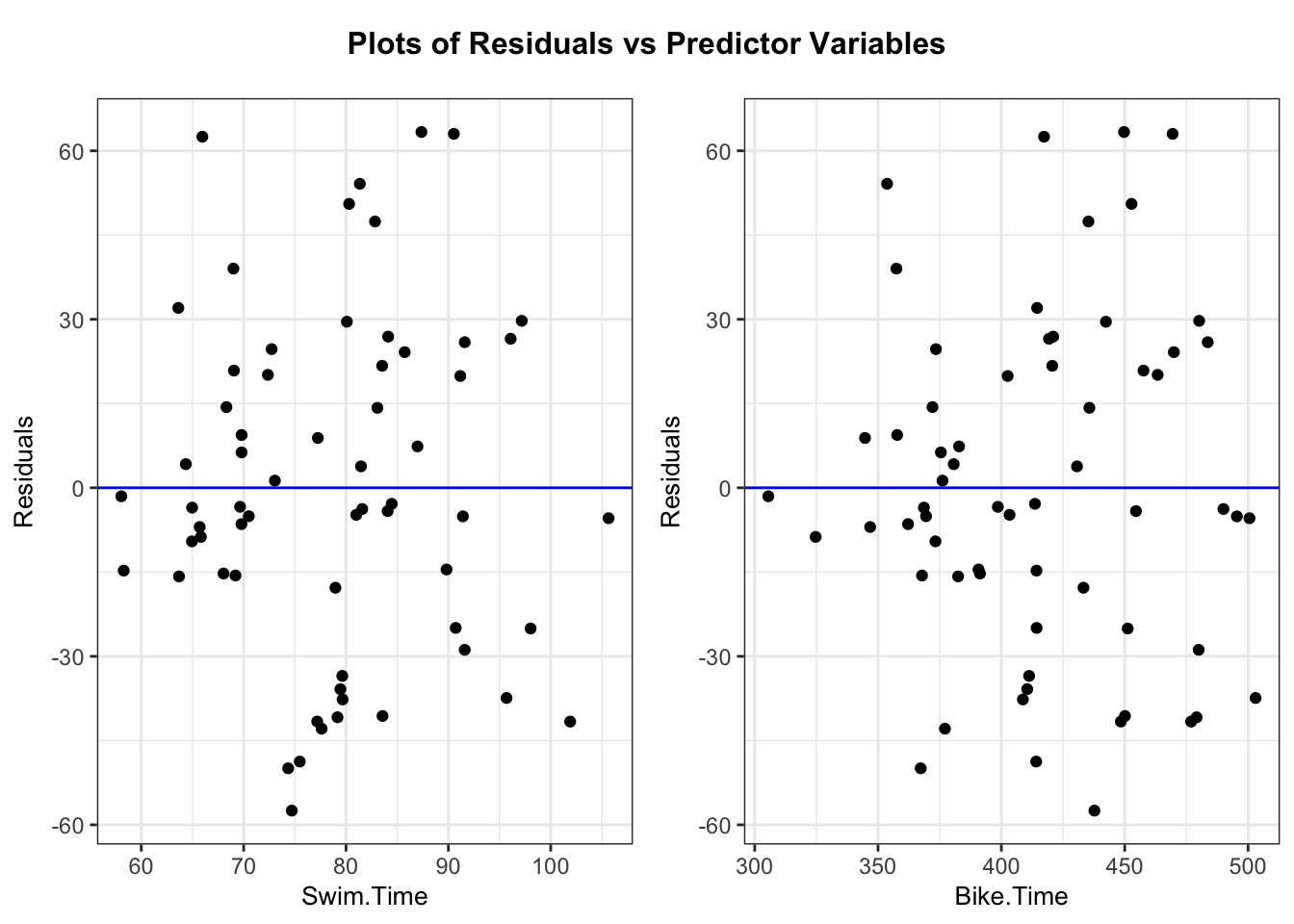
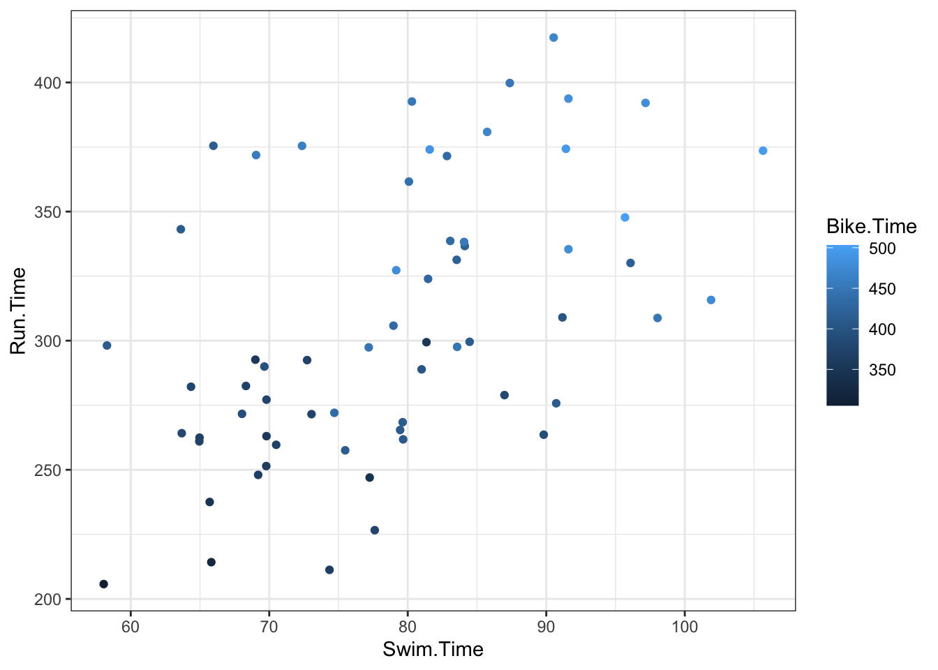
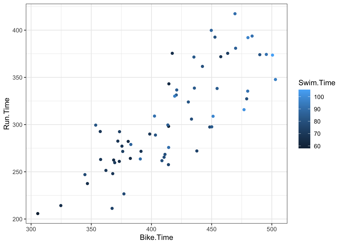
Using the 2022 Women’s Lake Placid Ironman data, we fit a regression model using run time as the response variable and swim and bike times as the explanatory variables. After adjusting for bike time, each minute increase of swim time was associated with a -0.38 minute increase in run time with a 95% interval of (-1.33, 0.58). After adjusting for swim time, each minute increase of bike time was associated with a 0.97 (0.75, 1.2) minute increase in run time. The model with swim and bike time accounted for 67% of the variability in run time.

3.3 ANOVA

When our explanatory variable is categorical with more than 2 levels, we can fit a regression model that will often be referred to as an ANOVA model.

To fit this model, we do the following

Choose one level to be the reference level (by default R will choose the level that comes first alphabetically)
Create indicator variables for all the other levels, i.e. \[ \mathrm{I}(\mbox{level for observation $i$ is $<$level$>$}) = \left\{ \begin{array}{ll} 1 & \mbox{if level for observation $i$ is $<$level$>$} \\ 0 & \mbox{otherwise} \end{array} \right. \]
Fit a regression model using these indicators.

Most statistical software will perform these actions for you, but it is useful to know this is what is happening.

Summary statistics

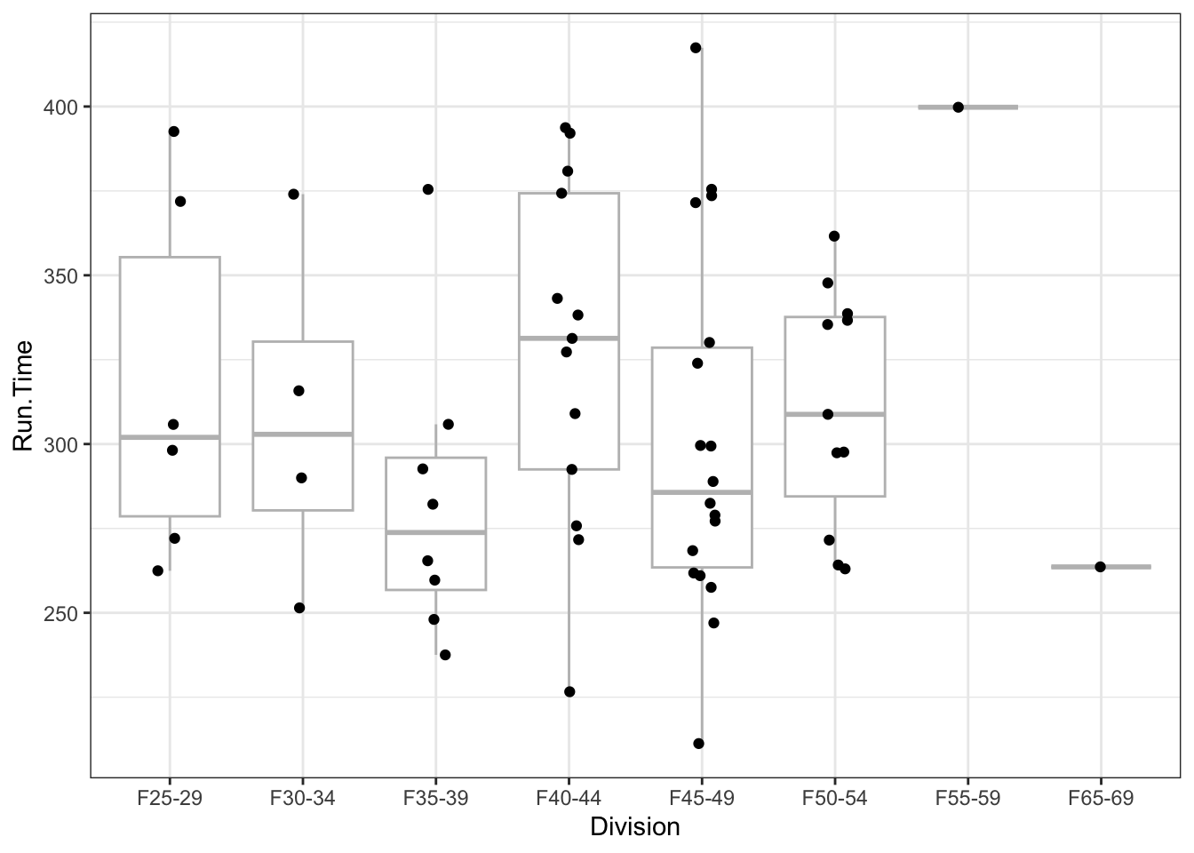
d |> group_by(Division) |> 
  summarize(
    n    = n(),
    mean = mean(Run.Time),
    sd   = sd(Run.Time)
  )

# A tibble: 9 × 4
  Division     n  mean    sd
  <chr>    <int> <dbl> <dbl>
1 F25-29       6  317. 53.3 
2 F30-34       4  308. 51.5 
3 F35-39       8  283. 43.6 
4 F40-44      13  327. 51.2 
5 F45-49      18  301. 53.9 
6 F50-54      11  311. 35.1 
7 F55-59       1  400. NA   
8 F65-69       1  264. NA   
9 FPRO         2  210.  6.00

ggplot(d |> filter(Division != "FPRO"),
       aes(x = Division, y = Run.Time)) +
  geom_boxplot(outliers = FALSE, color = "gray") +
  geom_jitter(width = 0.1)

m <- lm(Run.Time ~ Division, data = d |> filter(Division != "FPRO"))
summary(m)


Call:
lm(formula = Run.Time ~ Division, data = filter(d, Division != 
    "FPRO"))

Residuals:
     Min       1Q   Median       3Q      Max 
-100.808  -35.221   -2.173   26.991  115.983 

Coefficients:
               Estimate Std. Error t value Pr(>|t|)    
(Intercept)     317.164     19.924  15.918   <2e-16 ***
DivisionF30-34   -9.351     31.503  -0.297    0.768    
DivisionF35-39  -33.816     26.358  -1.283    0.205    
DivisionF40-44   10.260     24.087   0.426    0.672    
DivisionF45-49  -15.747     23.007  -0.684    0.497    
DivisionF50-54   -6.017     24.769  -0.243    0.809    
DivisionF55-59   82.619     52.715   1.567    0.123    
DivisionF65-69  -53.564     52.715  -1.016    0.314    
---
Signif. codes:  0 '***' 0.001 '**' 0.01 '*' 0.05 '.' 0.1 ' ' 1

Residual standard error: 48.8 on 54 degrees of freedom
Multiple R-squared:  0.143, Adjusted R-squared:  0.03195 
F-statistic: 1.288 on 7 and 54 DF,  p-value: 0.274

3.3.1 F-test

When evaluating the statistical support for including a categorical variable with more than 2 levels, we use an F-test.

The hypotheses in an F-test are

$H_0: \mu_g = \mu$ (the means in all the groups are the same)
$H_1: \mu_g \ne \mu_{g'}$ for some $g,g'$ (at least one mean is different)

anova(m)

Analysis of Variance Table

Response: Run.Time
          Df Sum Sq Mean Sq F value Pr(>F)
Division   7  21469  3067.1  1.2877  0.274
Residuals 54 128622  2381.9

drop1(m, test = "F")

Single term deletions

Model:
Run.Time ~ Division
         Df Sum of Sq    RSS    AIC F value Pr(>F)
<none>                128622 489.52               
Division  7     21469 150091 485.10  1.2877  0.274

# Alternatively fit two models and compare
m0 <- lm(Run.Time ~ 1, data = d |> filter(Division != "FPRO"))
anova(m0, m)

Analysis of Variance Table

Model 1: Run.Time ~ 1
Model 2: Run.Time ~ Division
  Res.Df    RSS Df Sum of Sq      F Pr(>F)
1     61 150091                           
2     54 128622  7     21469 1.2877  0.274

Interpretation

cbind(coef(m)[c(1, 3)], confint(m)[c(1, 3), ]) # divide by 60 to get hours

                            2.5 %    97.5 %
(Intercept)    317.16389 277.2179 357.10992
DivisionF35-39 -33.81597 -86.6596  19.02766

summary(m)$r.squared

[1] 0.1430418

anova(m)$`Pr(>F)`[1]

[1] 0.2740308

Using the 2022 Women’s Lake Placid Ironman data, we fit a regression model using run time as the response variable and age division as the explanatory variable. The mean run time for the F25-29 division was 5.3 hours with a 95% interval of (4.6, 6). There is evidence of a difference in mean run time amongst the divisions (ANOVA F-test p=0.27). The estimated difference in run time for the F25-29 division minus the F35-39 division was 34 (-19, 87) minutes. The model with division accounted for 14% of the variability in run time.