8  Win-Tie-Loss Models

library("MASS")    # polr: ordinal logistic regression model
library("ordinal") # clm: ordinal logistic regression model
library("dplyr")

Attaching package: 'dplyr'
The following object is masked from 'package:ordinal':

    slice
The following object is masked from 'package:MASS':

    select
The following objects are masked from 'package:stats':

    filter, lag
The following objects are masked from 'package:base':

    intersect, setdiff, setequal, union
library("tidyr")
library("ggplot2"); theme_set(theme_bw())
library("DT")

When sports allow ties, the statistical model used should accommodate the ordinal nature of the data. Namely, \[ \mbox{Win} > \mbox{Tie} > \mbox{Loss} \] We can extend the win-loss logistic regression model to accommodate the possibility of a Tie.

8.1 Model

To construct an ordinal logistic regression model, we will start with a latent-variable representation of the logistic regression model. We will then add additional cut-points to represent the different possible game outcomes.

8.1.1 Latent Variable Logistic Regression

Recall that our win-loss logistic regression model is \[H_g\stackrel{ind}{\sim} Ber(\pi_g) \quad \mbox{logit}(\pi_g) = \zeta + \theta_{H[g]} - \theta_{A[g]}\] where

  • \(H_g\) is an indicator that the home team won game \(g\) (0 if home team lost, 1 if home team won),
  • \(\zeta\) is the home advantage, and
  • \(\theta_t\) is the strength of team \(t\).

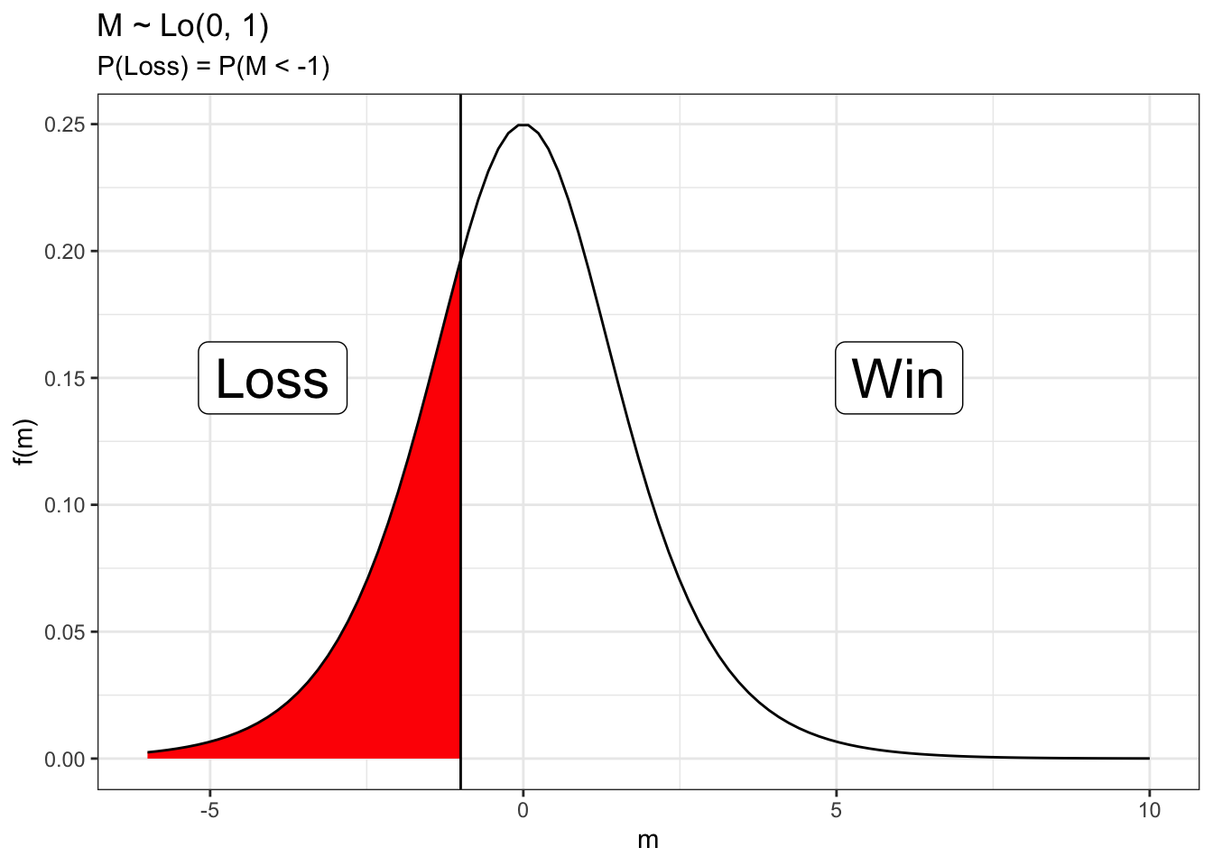
An equivalent way to express this model introduces a latent variable \(M_g^\zeta\) with a logistic distribution. Given this latent variable, the outcome is deterministic. Namely, \[H_g = \mathrm{I}(M_g^\zeta > 0)\] Latent variables often have a real-world interpretation. In this case, \(M_g^\zeta\) is related to the margin of victory. If the margin of victory is greater than 0, the home team wins and the home win indicator is 1, i.e. \(H_g = 1\).

In the implementation of the model used below, we will need a transformed version of this latent variable \(M_g = M_g^\zeta - \zeta\). With this transformed version we have

\[H_ g = \mathrm{I}(M_g > -\zeta)\] For logistic regression, \(M_g\) has a logistic distribution. For identifiability reasons, this distribution has a fixed scale parameter and, by convention, is often set to 1. Thus, \[M_g \stackrel{ind}{\sim} Lo(\mu_g, 1).\] The mean of this distribution is our typical model using home advantage and team strengths. \[\mu_g = E[M_g] = \theta_{H[g]} - \theta_{A[g]}.\] We can show \(\pi_g = P(M_g > -\zeta)\) and thus the latent variable representation is exactly the same as the typical representation we have used previously. Changing \(E[\mu_g]\) changes where the logistic distribution is centered on the number line and therefore the \(P(M_g > -\zeta)\).

h <- 0.15 # height of labels

g <- ggplot(data.frame(x = c(-6, 10)),
       aes(x = x)) +
  stat_function(fun = dlogis, 
                xlim = c(-6, -1), geom = "area", fill = "red") +
  stat_function(fun = dlogis) +
  geom_vline(xintercept = -1) +
  labs(
    x = "m",
    y = "f(m)",
    title = "M ~ Lo(0, 1)",
    subtitle = "P(Loss) = P(M < -1)"
  ) +
  annotate("label",  6, h, label = "Win",  size = 8) +
  annotate("label", -4, h, label = "Loss", size = 8) 

g

In this figure, we can see that the estimated home advantage can be alternatively interpreted as the threshold (or cutpoint) for change from a loss to a win. Values for \(M_g\) below the threshold result in a loss while values above the threshold result in a win.

8.1.2 Ordinal Logistic Regression

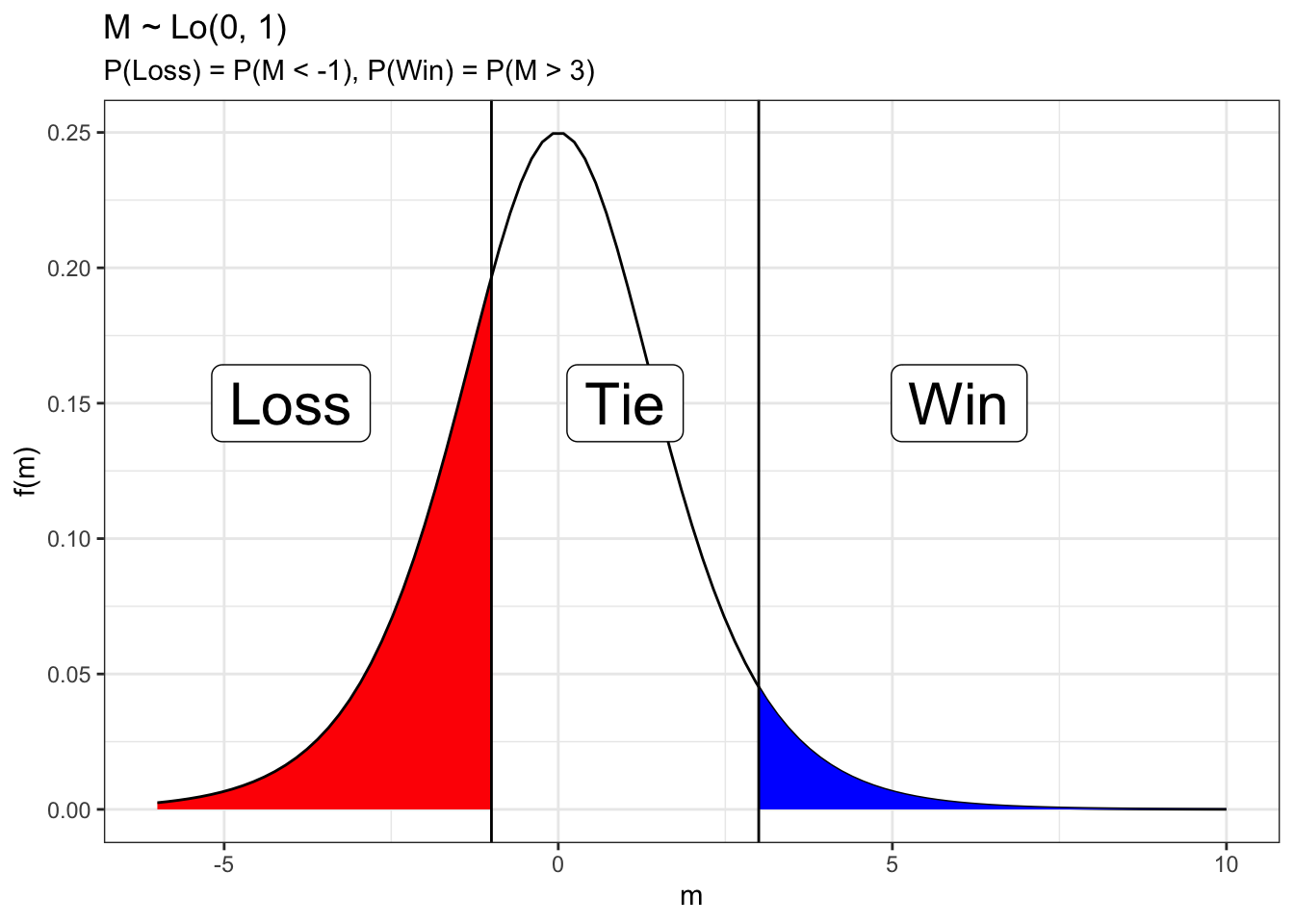
To account for ties in addition to wins and losses, we can include an additional threshold to separate ties from wins.
Modifying the above picture it may look something like this.

tw <- 3 # tie-win threshold

g +
  stat_function(fun = dlogis, 
                xlim = c(tw, 10), geom = "area", fill = "blue") +
  geom_vline(xintercept = tw) +
  annotate("label", mean(c(-1, tw)), h, label = "Tie", size = 8) +
  labs(
    subtitle = "P(Loss) = P(M < -1), P(Win) = P(M > 3)"
  )

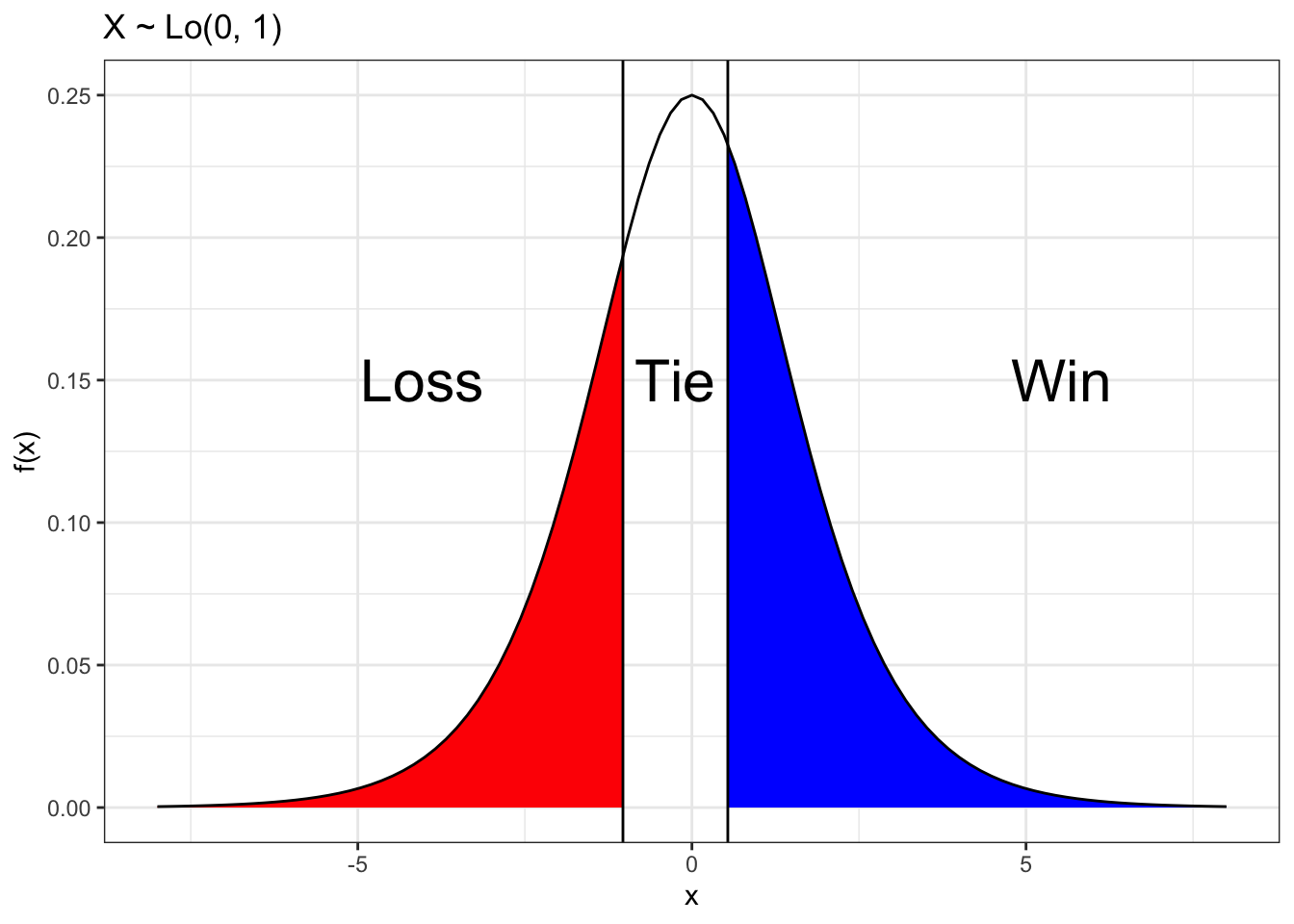
So we ordinal logistic regression model has a similar latent variable \[M_g \stackrel{ind}{\sim} Lo(\theta_{H[g]} - \theta_{A[g]}, 1)\] and two thresholds \[\mbox{R}_g = \left\{ \begin{array}{ll} Loss & M_g < \zeta_1 \\ Tie & \zeta_1 < M_g < \zeta_2 \\ Win & \zeta_2 < M_g \end{array} \right.\] \(R_g\) is an ordinal categorical variable that indicates the result of the game (loss, tie, or win) from the home team’s perspective. The parameters in this model are

  • \(\theta_t\): strength of team \(t\),
  • \(\zeta_1\): threshold separating loss from tie, and
  • \(\zeta_2\): threshold separating tie from win.

The thresholds are common to all games and teams. The thresholds are related to home advantage since, as the values of these thresholds get more negative, the probability the home team wins increases.

To calculate loss, tie, and win probabilities, we calculate the probability that the latent variable \(M_g\) falls within the three intervals: \((-\infty, \zeta_1)\), \((\zeta_1, \zeta_2)\), and \((\zeta_2,\infty)\), respectively.

8.2 Examples

8.2.1 2024-2025 Serie A

serieA_raw <- read.csv("data/serieA_2024-2025.csv")

serieA_teams <- with(serieA_raw, sort(unique(c(Home, Away))))

serieA <- serieA_raw |>
  mutate(
    home_result = case_when(
      Home_Score >  Away_Score ~ "Win",
      Home_Score == Away_Score ~ "Tie",
      Home_Score <  Away_Score ~ "Loss"
    ),
    
    home_result = factor(home_result,
                         levels = c("Loss", "Tie", "Win"), # order matters
                         ordered = TRUE), # needed for ordinal regression
    
    Home = factor(Home, levels = serieA_teams),
    Away = factor(Away, levels = serieA_teams)
  )

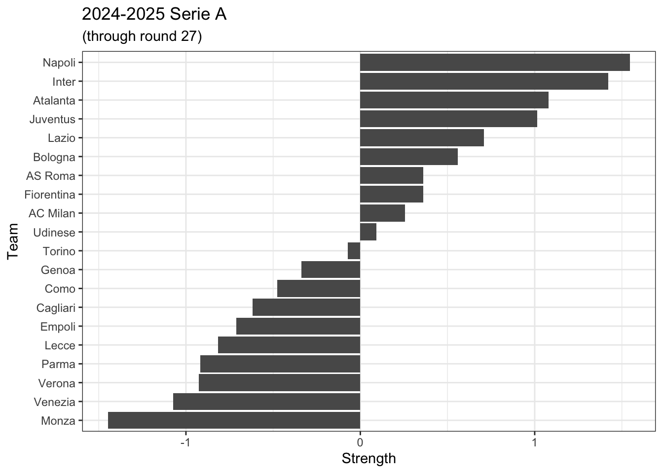
When we construct the ordered factor of loss-tie-win, we put it in order from loss to win. This results in team strengths where higher numbers indicate stronger teams.

Let’s check records first.

serieA |> 
  pivot_longer(
    cols = c("Home", "Away"),
    names_to = "Location",
    values_to = "Team"
  ) |>
  group_by(Team) |>
  summarize(
    n = n(),
    win = sum(
      (home_result == "Win" & Location == "Home") |
        (home_result == "Loss" & Location == "Away")
    ),
    tie = sum(home_result == "Tie"),
    loss = n - win - tie,
    points = 3 * win + tie
  ) |>
  arrange(desc(points)) |>
  datatable(filter = "top")

It looks like everybody has at least one win, one tie, and one loss so we should be able to identify the parameters.

Since this is league where everybody plays everybody else and we have 27 rounds of competitions, the graph is going to be very well connected.

Let’s construct out model matrix.

construct_model_matrix <- function(d, homeCol = "home", awayCol = "away") {
  n_games <- nrow(d)
  n_teams <- length(unique(unlist(d[, homeCol], d[, awayCol])))
  
  m <- matrix(0, 
              nrow = n_games, 
              ncol = n_teams)
  
  for (g in 1:n_games) {
    m[g, as.numeric(d[g, homeCol])] <-  1
    m[g, as.numeric(d[g, awayCol])] <- -1
  }
  
  return(m)
}

X <- construct_model_matrix(serieA, "Home", "Away")

Check model matrix

dim(X) # ngames x nteams
[1] 270  20
table(X)
X
  -1    0    1 
 270 4860  270 
all(rowSums(X) == 0)
[1] TRUE
all(rowSums(abs(X)) == 2)
[1] TRUE
colSums(X)
 [1]  1  1 -1  1  1 -1 -1  1  1 -1  1 -1 -1  1 -1  1 -1  1 -1 -1

Fit ordinal logistic regression model.

m <- polr(serieA$home_result ~ X, Hess = TRUE) # warning is expected
Warning in polr(serieA$home_result ~ X, Hess = TRUE): design appears to be
rank-deficient, so dropping some coefs
summary(m)
Call:
polr(formula = serieA$home_result ~ X, Hess = TRUE)

Coefficients:
       Value Std. Error  t value
X1   1.18262     0.5506  2.14799
X2   1.28796     0.5725  2.24980
X3   2.00518     0.5764  3.47851
X4   1.48410     0.5694  2.60664
X5   0.30882     0.5640  0.54757
X6   0.44888     0.5677  0.79068
X7   0.21451     0.5617  0.38192
X8   1.28688     0.5737  2.24306
X9   0.58893     0.5585  1.05444
X10  2.34810     0.5950  3.94618
X11  1.94026     0.5582  3.47616
X12  1.63568     0.5708  2.86565
X13  0.11183     0.5646  0.19809
X14 -0.51892     0.5755 -0.90162
X15  2.47146     0.6018  4.10682
X16  0.01012     0.5727  0.01767
X17  0.85384     0.5543  1.54033
X18  1.01908     0.5598  1.82046
X19 -0.14775     0.5527 -0.26733

Intercepts:
         Value   Std. Error t value
Loss|Tie -1.0323  0.1527    -6.7611
Tie|Win   0.5373  0.1423     3.7744

Residual Deviance: 496.1578 
AIC: 538.1578 

Compute team strengths

teams <- data.frame(
  names    = serieA_teams,
  strength = c(coef(m), 0)
) |>
  mutate(
    strength = strength - mean(strength),
    names = factor(names, levels = names[order(strength)])
  ) |>
  arrange(desc(names))

teams |>
  datatable(filter = "top")

Plot team strengths

ggplot(teams,
       aes(
         x = strength,
         y = names
       )) +
  geom_bar(stat = "identity") +
  labs(
    x = 'Strength',
    y = 'Team',
    title = '2024-2025 Serie A',
    subtitle = '(through round 27)'
  )

To calculate probabilities we need to utilize the intercepts from the model output.

m$zeta # thresholds
 Loss|Tie   Tie|Win 
-1.032252  0.537282 

These intercepts indicate the change-points when moving from a Loss to Tie to Win.

# Function to calculate probabilities
calculate_ordinal_probabilities <- function(mean, zeta) {
  p <- c(
    plogis(zeta[1] - mean),
    diff(plogis(zeta - mean)),
    plogis(zeta[2] - mean, lower.tail = FALSE)
  ) 
  
  names(p) <- c("loss", "tie", "win")
  
  return(p)
}

# Equal strength teams
calculate_ordinal_probabilities(0, m$zeta)
     loss       tie       win 
0.2626477 0.3685322 0.3688201 

We can visualize these probabilities using the logistic distribution and the areas under the curve.

ggplot(data.frame(x = c(-8, 8)),
       aes(x = x)) +
  stat_function(fun = dlogis, 
                xlim = c(-8, m$zeta[1]), 
                geom = "area", 
                fill = "red") +
  stat_function(fun = dlogis, 
                xlim = c(m$zeta[2], 8), 
                geom = "area", 
                fill = "blue") +
  stat_function(fun = dlogis) +
  geom_vline(xintercept = m$zeta[1]) +
  geom_vline(xintercept = m$zeta[2]) +
  labs(
    y = "f(x)",
    title = "X ~ Lo(0, 1)"
  ) +
  annotate("text",  m$zeta[2]+5,  0.15, label = "Win",  size = 8) +
  annotate("text",  m$zeta[1]-3,  0.15, label = "Loss", size = 8) +
  annotate("text",  mean(m$zeta), 0.15, label = "Tie",  size = 8) 

# Napoli v Inter
calculate_ordinal_probabilities(
  teams$strength[teams$names == "Napoli"] -
    teams$strength[teams$names == "Inter"], 
  m$zeta)
     loss       tie       win 
0.2394653 0.3625623 0.3979724 
# Napoli v Inter
calculate_ordinal_probabilities(
  teams$strength[teams$names == "Napoli"] -
    teams$strength[teams$names == "Monza"], 
  m$zeta)
      loss        tie        win 
0.01759073 0.06162130 0.92078797 

8.3 R packages

In this analysis, we utilized the polr() function from the MASS package since this package is installed by default when you install R.

The ordinal can also implement the ordinal logistic regression model using the clm() function.

mo <- ordinal::clm(serieA$home_result ~ X)
summary(mo)
formula: serieA$home_result ~ X

 link  threshold nobs logLik  AIC    niter max.grad cond.H 
 logit flexible  270  -248.08 538.16 4(0)  7.57e-08 3.1e+02

Coefficients: (1 not defined because of singularities)
    Estimate Std. Error z value Pr(>|z|)    
X1   1.18255    0.55057   2.148 0.031725 *  
X2   1.28817    0.57249   2.250 0.024441 *  
X3   2.00551    0.57647   3.479 0.000503 ***
X4   1.48435    0.56937   2.607 0.009133 ** 
X5   0.30868    0.56400   0.547 0.584168    
X6   0.44900    0.56772   0.791 0.429012    
X7   0.21487    0.56167   0.383 0.702052    
X8   1.28734    0.57373   2.244 0.024844 *  
X9   0.58919    0.55853   1.055 0.291472    
X10  2.34794    0.59503   3.946 7.95e-05 ***
X11  1.94024    0.55817   3.476 0.000509 ***
X12  1.63564    0.57079   2.866 0.004163 ** 
X13  0.11194    0.56457   0.198 0.842829    
X14 -0.51932    0.57557  -0.902 0.366920    
X15  2.47149    0.60180   4.107 4.01e-05 ***
X16  0.01056    0.57268   0.018 0.985285    
X17  0.85397    0.55433   1.541 0.123427    
X18  1.01946    0.55980   1.821 0.068591 .  
X19 -0.14806    0.55270  -0.268 0.788785    
X20       NA         NA      NA       NA    
---
Signif. codes:  0 '***' 0.001 '**' 0.01 '*' 0.05 '.' 0.1 ' ' 1

Threshold coefficients:
         Estimate Std. Error z value
Loss|Tie  -1.0323     0.1527  -6.761
Tie|Win    0.5373     0.1423   3.774

An appealing aspect of this package is the ability to fixed mixed effect ordinal regression models using the clmm() function.

8.4 Summary

The development here used the logistic distribution due to its relationship with logistic regression. An alternatively commonly used approach uses the normal distribution due to its relationship with probit regression.