Since we know that distance will affect the probability of making a field goal, we should adjust for distance when comparing the two kickers.
We have multiple ways of comparing the two, but one of the simplest is to conduct a logistic regression where the response is binary of whether or not the kick was made and the explanatory variables are distance, kicker, and the kicker distance interaction. The interaction is important because it allows the effect of distance on probability of making the field goal to be different for each kicker.
Here we have an interaction between a continuous variable (distance) and a categorical/binary variable (kicker). We could evaluate whether the interaction has support in the data by doing a statistical test. If we decide, based on that test or other expertise, that we would liek to include an interaction, then this model is equivalent to running a separate logistic regression for each kicker. Thus individual regression for each kicker with the sole explanatory variable being distance is reasonable.
Let \(Y_{i,p}\) be in indicator that kick \(i\) by player \(p\) was made. An independent (or individual or separate) logistic regression for each kicker with distance as the explanatory variable would look like
\[Y_{i,p} \stackrel{ind}{\sim} Ber(\pi_{i,p}), \quad
\mbox{logit}(\pi_{ip}) = \beta_{0,p} + \beta_{1,p} d_{i,p}
\] where \(d_{i,p}\) is the distance of kick \(i\) by player \(p\).
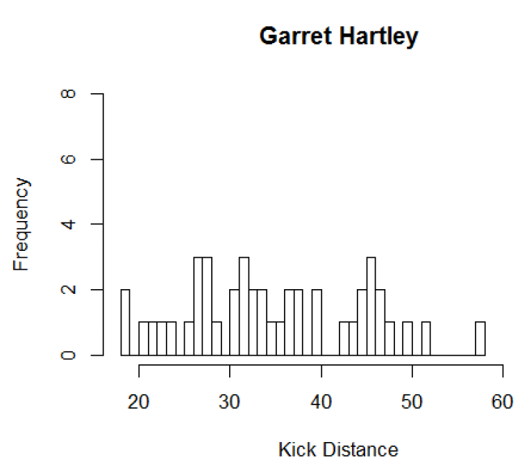
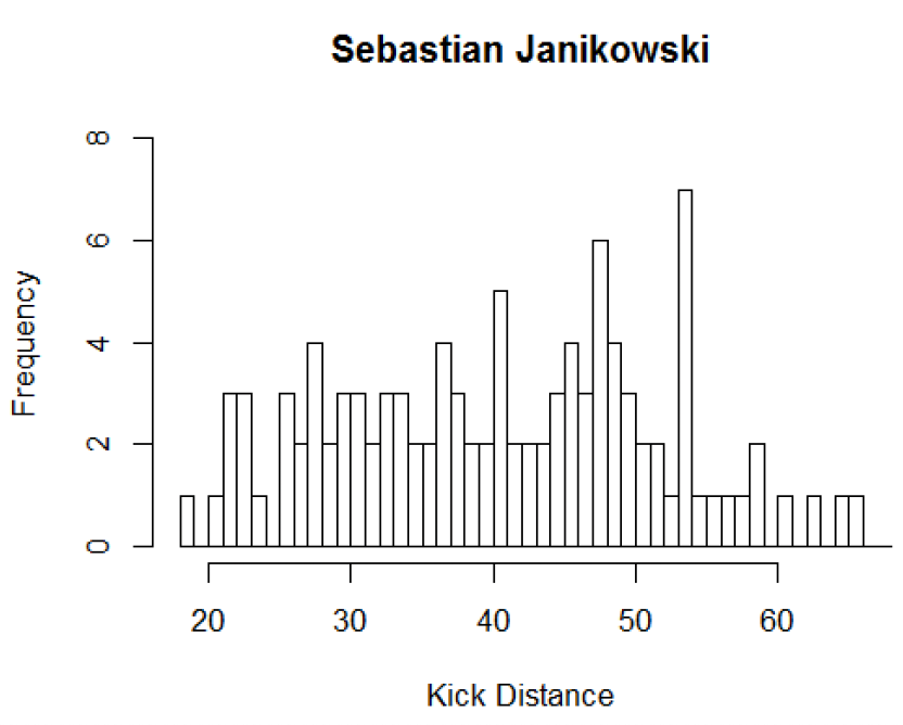
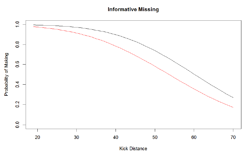
In all of the following figures Janikowski is in black and Hartley is in red.
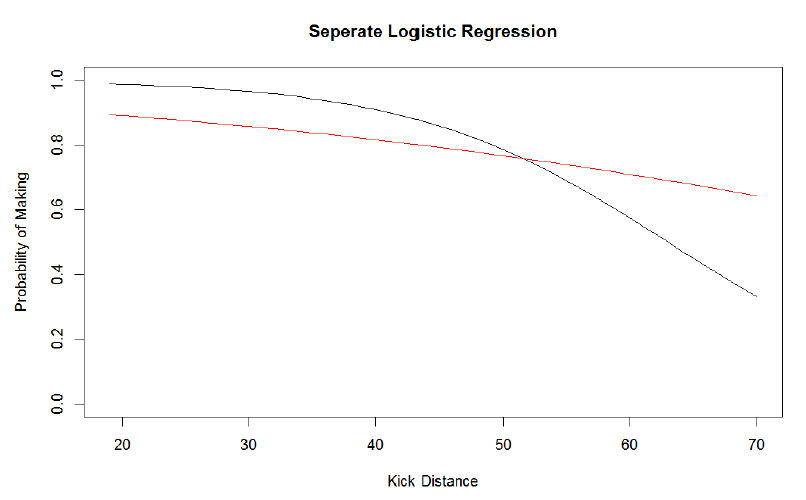
This plot suggests that Janikowski is a better field goal kicker but his probability to make field goals is highly affected by distance while Hartley’s probability is more consistent across the distances. Knowledge of these two kickers will tell you that this is not the case since Janikowski is a renowned long distance kicker.
13.1.2 Hierarchical Regression Model
The main reason the analysis suggests the opposite is true is because we do not have much data on long distance kicks for Hartley. Using a random (or mixed) effects model can help to borrow strength across NFL kickers to better estimate Hartley (and other kickers effectiveness). In this case, a random slope model would add an additional assumption to the logistic regression model above, namely
\[\left[ \begin{array}{c}\beta_{0,p} \\ \beta_{1,p} \end{array}\right]
\stackrel{ind}{\sim}
N\left(\left[ \begin{array}{c}\beta_{0} \\ \beta_{1} \end{array}\right],
\left[ \begin{array}{cc}\sigma^2_0 & \rho\sigma_0\sigma_1 \\
\rho\sigma_0\sigma_1 & \sigma^2_1\end{array}\right]
\right)
\] where this is a bivariate normal distribution with, across all kickers,
\(\beta_0\) is the mean intercept,
\(\beta_1\) is the mean slope,
\(\sigma_0\) is the standard deviation in the intercept,
\(\sigma_1\) is the standard deviation in the slope, and
\(\rho\) is the correlation between the intercepts and slopes.
The key with this model is that all intercepts and slopes are shrunk back to the overall mean intercept and slope across all kickers. The amount that these are shrunk is inversely related to how much data there is to support the individual player abilities. Thus, players with a lot of data will not be shrunk much while players with a lot of data will be shrunk a lot.
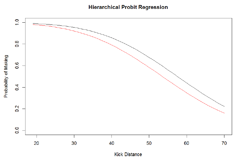
The following is the estimate of Hartley (red) and Janikowski (black) probability of making a kick as a function of distance.
This analysis is intuitively reasonable since Janikowski appears to be the better kicker at all distances and the effect of distance being less for Janikowski compared to Hartley.
13.1.3 Missing Model
This is actually a case of missing data. The data that are missing are kicks at longer distances (for both kickers). There are 4th downs (and some non 4th downs) where it would make sense to try for a kick, e.g. it is late in the game and the team is down by 3 or fewer points. In these situations, the coach makes a decision whether to have the kicker attempt a field goal or not. From our knowledge of the kickers, we know that Janikowski is (relatively) often asked to attempt long distance kicks compared to Hartley. The reason Janikowski is asked to attempt these kicks and Hartley is not is because the coach believes Janikowski has a (relatively) high probability of making the kick while Hartley does not.
Thus, we can build an additional model for the probability of an attempt. If this probability of an attempt includes the probability of making the field goal, then the model can learn about the probability of making the field goal by whether or not the coach asks the kicker to attempt the kick.
Let \(A_{j,p}\) be an indicator that player \(p\) is asked to attempt a field goal on play \(j\). A model could be
\[A_{j,p} \stackrel{ind}{\sim} Ber(\theta_{j,p}), \quad
\mbox{logit}(\theta_{j,p}) = \alpha_{0,p} + \alpha_{1,p} \mbox{logit}(\pi_{j,p})
\] where we would likely have a hierarchical model for the \(\alpha\)s.
Incorporating this into the analysis provides an informative missingness model. The estimated probability for Janikowski (black) and Hartley (red) from this model is given below.