Warning: package 'purrr' was built under R version 4.4.1
── Attaching core tidyverse packages ──────────────────────── tidyverse 2.0.0 ──
✔ dplyr     1.1.4.9000     ✔ readr     2.1.5
✔ forcats   1.0.0          ✔ stringr   1.5.1
✔ ggplot2   3.5.1          ✔ tibble    3.2.1
✔ lubridate 1.9.3          ✔ tidyr     1.3.1
✔ purrr     1.0.4
── Conflicts ────────────────────────────────────────── tidyverse_conflicts() ──
✖ dplyr::filter() masks stats::filter()
✖ dplyr::lag()    masks stats::lag()
ℹ Use the conflicted package (<http://conflicted.r-lib.org/>) to force all conflicts to become errors
library("ggResidpanel")
set.seed(20250212) # Reproducible simulations
5.1 Model
Let \(Y_i\) be the count out of \(n_i\) attempts where each attempt is independent and there is a common probability of success \(\pi_i\). We assume \[Y_i \stackrel{ind}{\sim} Bin(n_i, \pi_i).\] A special case is when \(n_i = 1\) and \(Y_i\) is a binary (Bernoulli) variable.
If, for each \(i\) we have a collection of explanatory variables \(X_{i,1}, \ldots X_{i,p}\), then a logistic regression model assumes \[
\mbox{logit}(\pi_i)=\mbox{log}\left( \frac{\pi_i}{1-\pi_i} \right) =
\eta_i =
\beta_0 + \beta_1 X_{i,1} + \beta_2 X_{i,2} + \cdots +\beta_p X_{i,p}
\]
where the logistic function of \(\eta_i\) is \[
\pi_i = f(\eta_i)
= \frac{e^{\eta_i}}{1+e^{\eta_i}}
= \frac{1}{1+e^{-\eta_i}}.
\]
Some like to call this the expit() function (since it is the opposit of the logit() function above), so we will use this convention in the code
expit <-function(eta) {1/ (1+exp(-eta))}
5.1.1 Interpretation
When \(X_{i,j} = 0\) for all \(j\), then \[
E[Y_i|X_{i,1} = 0, \ldots,X_{i,p} = 0] = \pi_i = \frac{1}{1+e^{-\beta_0}}
\]
thus \(\beta_0\) determines the probability of success when the explanatory variables are all zero.
The odds of success when \(X_{i,j} = x_j\) is \[
\frac{\pi_1}{1-\pi_1} = e^{\beta_0+\beta_1x_1 + \cdots \beta_p x_p}.
\]
The probability of success when \(X_1 =x_1 + 1\) and the remainder are left at \(X_{i,j} =x_j\) is \[
\frac{\pi_2}{1-\pi_2} = e^{\beta_0+\beta_1(x_1+1) + \cdots \beta_p x_p}
= e^{\beta_0+\beta_1x_1 + \cdots \beta_p x_p}e^{\beta_1} =
\frac{\pi_1}{1-\pi_1} e^{\beta_1}.
\]
Thus, the multiplicative change in the odds for a 1 unit increase in \(X_1\) is \[
\frac{\frac{\pi_2}{1-\pi_2}}{\frac{\pi_1}{1-\pi_1}}
= e^{\beta_1}
\]
This is also referred to as an odds ratio.
5.2 WNBA Shooting
This kaggle competition provides data on plays in the WNBA during the 2021-2022 season. We’ll take a look at the field goal makes as our successes.
wnba_shots <-read_csv("data/wnba-shots-2021.csv") |>filter( !(grepl("Free Throw", shot_type)) ) |>mutate(# Calculate distance to the hoop which is apparently at (25, 0)# https://www.kaggle.com/datasets/mexwell/women-national-basketball-association-shotsdistance =sqrt((coordinate_x -25)^2+ (coordinate_y -0)^2) ) |>filter( !is.na(distance), !is.na(made_shot))
Rows: 41497 Columns: 16
── Column specification ────────────────────────────────────────────────────────
Delimiter: ","
chr  (5): desc, shot_type, shooting_team, home_team_name, away_team_name
dbl (10): game_id, game_play_number, shot_value, coordinate_x, coordinate_y,...
lgl  (1): made_shot

ℹ Use `spec()` to retrieve the full column specification for this data.
ℹ Specify the column types or set `show_col_types = FALSE` to quiet this message.
Due to the quote in Love Triangle about having shots incorrectly coded as 2-pointers or 3-pointers, we’ll take a look at points that may be incorrectly coded in these data.
We probably need to look into this more thoroughly before we conclude these data are incorrectly coded.
5.2.1 Sylvia Fowles probability vs distance
# Extract Sylvia Fowles shotsfowles_shots <- wnba_shots |># Description (typically) starts with who is shootingfilter(str_starts(desc, "Sylvia Fowles"))table(fowles_shots$made_shot) # response
FALSE  TRUE
  122   187
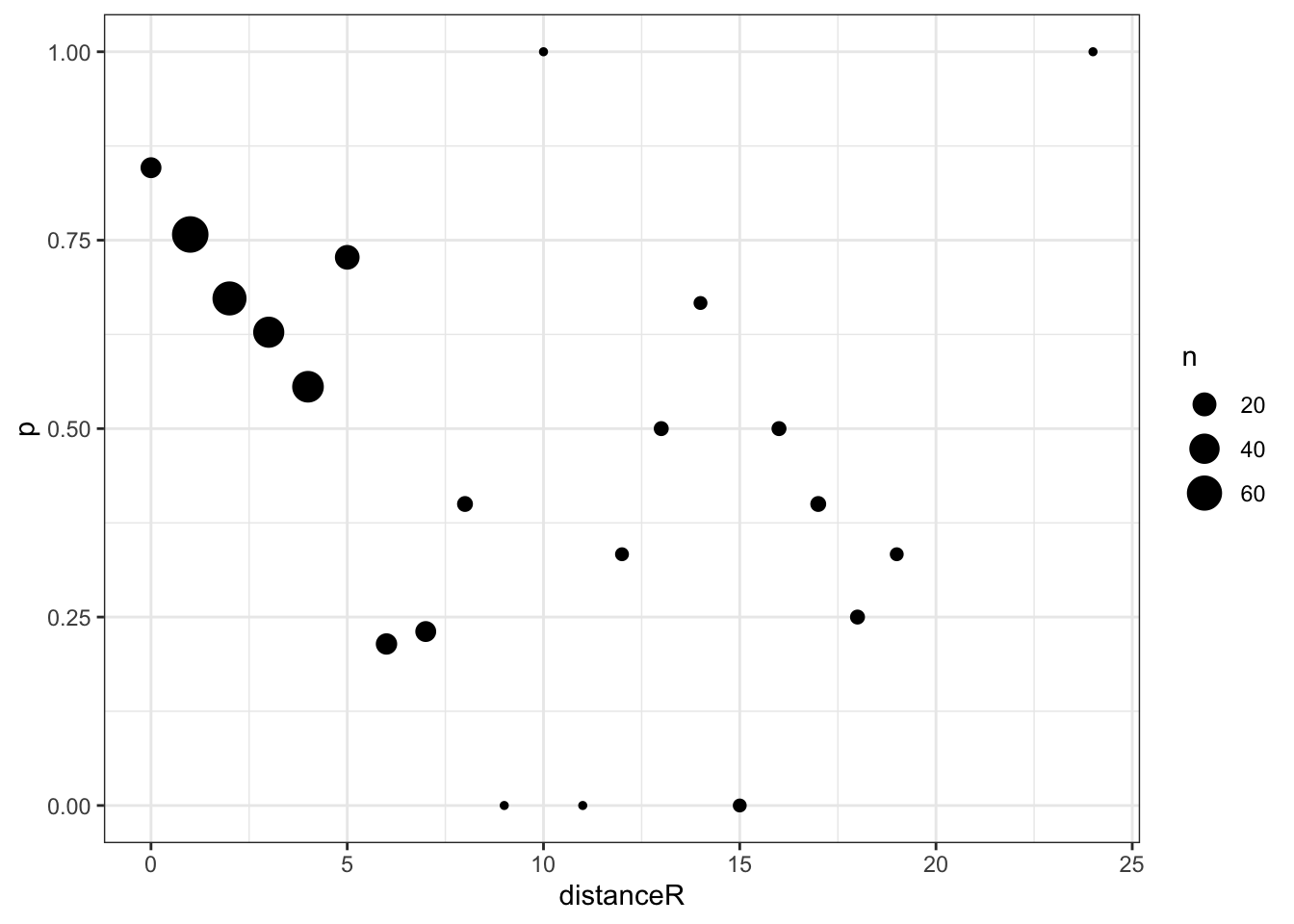
# For visualization purposes, aggregate shots by rounding to the nearest footaggregate_fowles_shots <- fowles_shots |>mutate(distanceR =round(distance) ) |>group_by(distanceR) |>summarize(n =n(),y =sum(made_shot), # TRUE gets converted to 1 and FALSE to 0p = y / n )g <-ggplot(aggregate_fowles_shots,aes(x = distanceR, y = p, size = n)) +geom_point()g
m <-glm(made_shot ~ distance, # made_shot data = fowles_shots,family ="binomial")
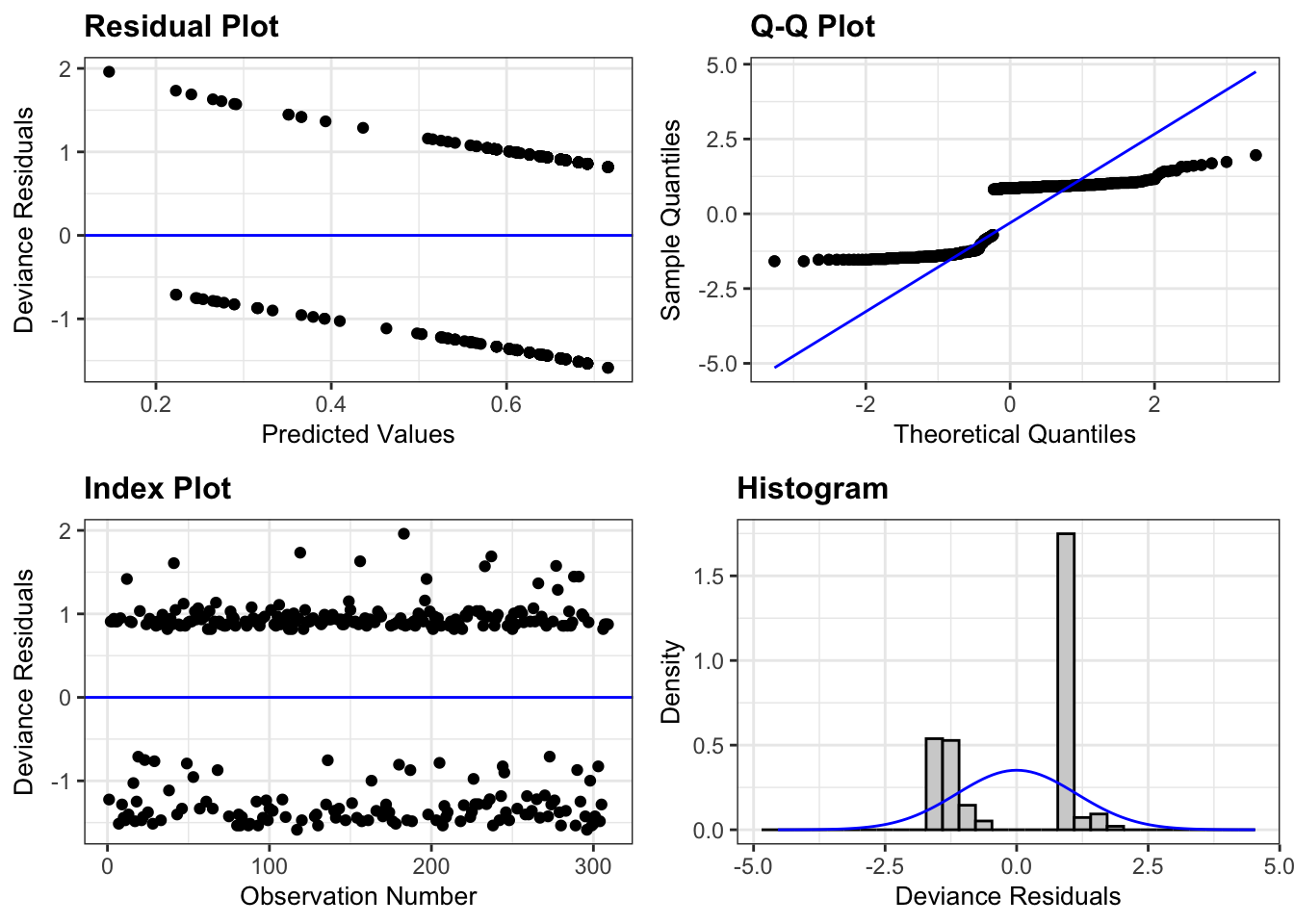
resid_panel(m)
summary(m)
Call:
glm(formula = made_shot ~ distance, family = "binomial", data = fowles_shots)

Coefficients:
            Estimate Std. Error z value Pr(>|z|)
(Intercept)  0.92302    0.17341   5.323 1.02e-07 ***
distance    -0.11297    0.02924  -3.863 0.000112 ***
---
Signif. codes:  0 '***' 0.001 '**' 0.01 '*' 0.05 '.' 0.1 ' ' 1

(Dispersion parameter for binomial family taken to be 1)

    Null deviance: 414.59  on 308  degrees of freedom
Residual deviance: 397.80  on 307  degrees of freedom
AIC: 401.8

Number of Fisher Scoring iterations: 4
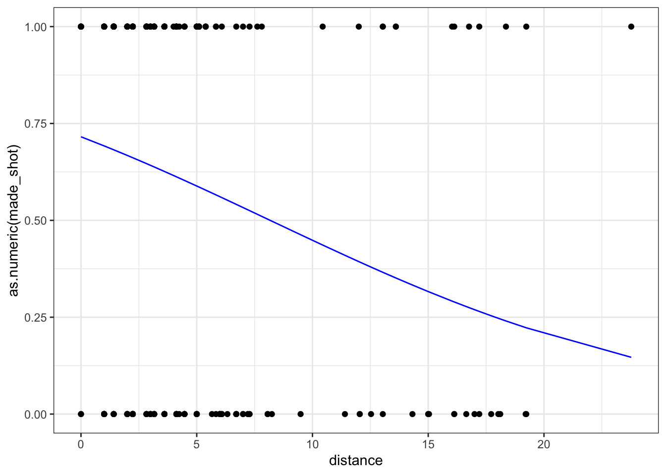
We ran a logistic regression using made shot as a success and distance from the hoop as the explanatory variable. According to the model, the probability of making a shot at a distance of 0 is
0.72 with a 95% confidence interval of (0.64, 0.78). For each additional foot away from the hoop the odds of making the shot is multiplied by 0.89 with a 95% confidence interval of (0.84, 0.94).
# Create data frame with fitted valuesfowles_fitted <- fowles_shots |>mutate(p =predict(m, type ="response"))ggplot(fowles_fitted,aes(x = distance)) +geom_point(aes(y =as.numeric(made_shot))) +geom_line(aes(y = p), col ='blue') +ylim(0, 1)
# A tibble: 2 × 4
  player            n     y     p
  <chr>         <int> <int> <dbl>
1 Sue Bird        267   107 0.401
2 Sylvia Fowles   309   187 0.605
Here we see that Sylvia Fowles is the better field goal shooter by field goal percent. This is consistent (although the numbers are somewhat different) with the WNBA 2021 Shooting Statistics.
We could fit a comparison of two binomial proportions.
We ran a logistic regression using the number of made shots out of the total and used player (Sylvia Fowles vs Sue Bird) as the explanatory variable. According to the model, the probability of making a shot for Sue Bird is 0.4 with a 95% confidence interval of (0.34, 0.46) and the multiplicative effect on log odds for Sylvia Fowles compared to Sue Bird is 2.29 with a 95% confidence interval of (1.64, 3.21).
We likely expect that distance will affect the probability of making a shot as we saw previously. So let’s include distance in our model.
mPD <-glm(made_shot ~ player + distance,data = two_player_shots,family ="binomial")summary(mPD)
Call:
glm(formula = made_shot ~ player + distance, family = "binomial",
    data = two_player_shots)

Coefficients:
                    Estimate Std. Error z value Pr(>|z|)
(Intercept)          0.51006    0.31922   1.598   0.1101
playerSylvia Fowles  0.11039    0.28761   0.384   0.7011
distance            -0.04398    0.01416  -3.105   0.0019 **
---
Signif. codes:  0 '***' 0.001 '**' 0.01 '*' 0.05 '.' 0.1 ' ' 1

(Dispersion parameter for binomial family taken to be 1)

    Null deviance: 798.26  on 575  degrees of freedom
Residual deviance: 764.33  on 573  degrees of freedom
AIC: 770.33

Number of Fisher Scoring iterations: 4
When we do not include distance in the model, it appears that Sylvia Fowles is the better shooter. When distance is included in the model, it appears that there is no evidence of a difference in field goal percentage between Sylvia Fowles and Sue Bird (p = 0.7). This is an example of Simpson’s Paradox, i.e. our understanding of a relationship changes as we adjust for other explanatory variables.
We may expect further that the effect of distance will be different for Sylvia Fowles compared to Sue Bird since Sylvia Fowles is a 6’6” center while Sue Bird is 5’9” point guard. To allow for the effect of distance to depend on the player, we include an interaction between distance and player.
mPDI <-glm(made_shot ~ player * distance, # Note the * for the interactiondata = two_player_shots,family ="binomial")summary(mPDI)
Call:
glm(formula = made_shot ~ player * distance, family = "binomial",
    data = two_player_shots)

Coefficients:
                              Estimate Std. Error z value Pr(>|z|)
(Intercept)                  -0.004762   0.363577  -0.013  0.98955
playerSylvia Fowles           0.927781   0.402815   2.303  0.02127 *
distance                     -0.019103   0.016459  -1.161  0.24577
playerSylvia Fowles:distance -0.093863   0.033558  -2.797  0.00516 **
---
Signif. codes:  0 '***' 0.001 '**' 0.01 '*' 0.05 '.' 0.1 ' ' 1

(Dispersion parameter for binomial family taken to be 1)

    Null deviance: 798.26  on 575  degrees of freedom
Residual deviance: 756.00  on 572  degrees of freedom
AIC: 764

Number of Fisher Scoring iterations: 4
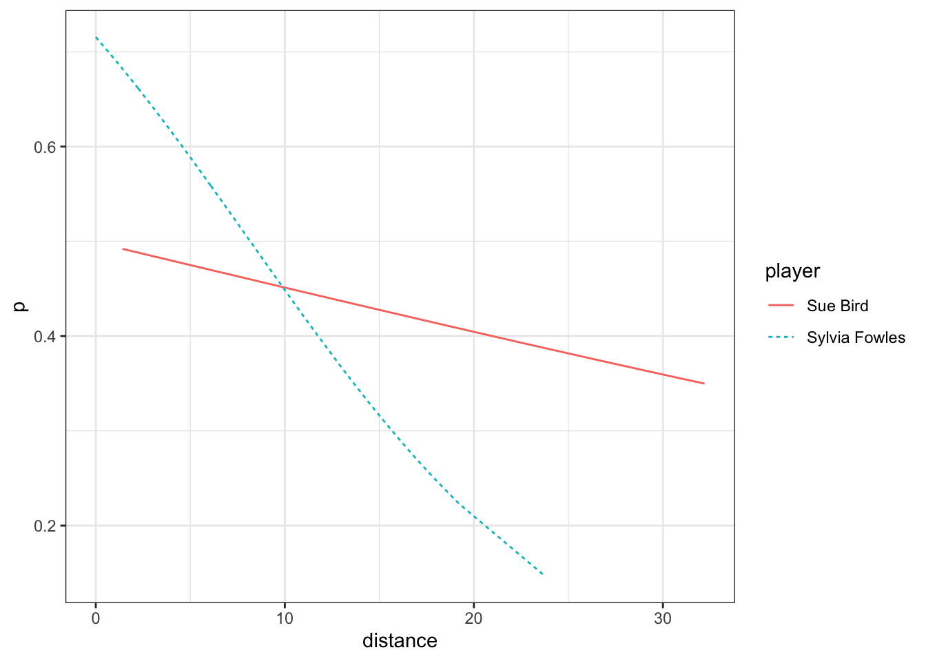
There is evidence that distance effects the two players differently (0.005). Rather than trying to directly interpret these coefficients, it is much more straightforward to plot the estimated probabilities as a function of distance.
two_player_shots_fitted <- two_player_shots |>mutate(p =predict(mPDI, type ="response") )ggplot(two_player_shots_fitted,aes(x = distance, y = p, color = player, group = player,linetype = player)) +geom_line()
This is certainly not the end of the story since probability might be a more complicated function of distance as we will see in the Golf putting example.
5.3 Golf putting
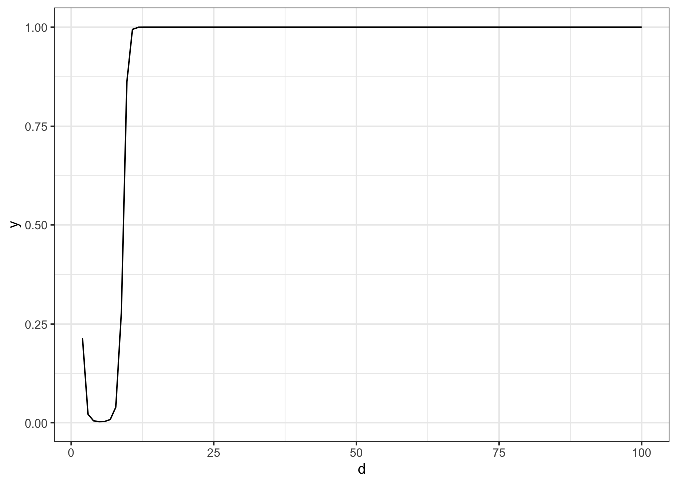
Fearing, Acimovic, and Graves (2011) fit a logistic regression model for the probability of making a putt as a function of the distance of the putt. The resulting function they used was
Huh?!?!?! This looks nothing like the authors estimated probability in Figure 3. I tried a variety of variations, e.g. using log base 10 and forgetting the negative sign in the exponential, but nothing seems to reproduce the plot the authors have.
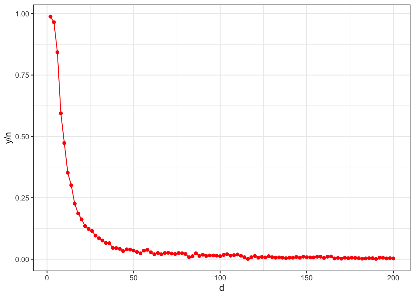
Since we don’t have their actual plot, I’ll try to recreate their data from Figure 2.
simulated_putts <-data.frame(n =1000, # I measured the height in the pdfp =c(12.9, 12.5, 11.1, 7.5, 5.8, 4.5, 3.7, 3, 2.5, 2.1, 1.8, 1.5,1.4, 1.2, 1.1, 1.0, .9, .8, .7, .6, .5, .5, .5, .5, rep(0.4, 6), rep(0.3, 10), rep(0.2, 16), rep(0.1, 26),rep(0.05, 18)) /13# total height) |>mutate(d =seq(2, by =2, length =n()),y =rbinom(n(), size = n, prob = p) )
Let’s plot the data to recreate Figure 2 from the paper.
ggplot(simulated_putts, aes(x = d, y = y / n)) +geom_point(color ='red') +geom_line(color ='red')
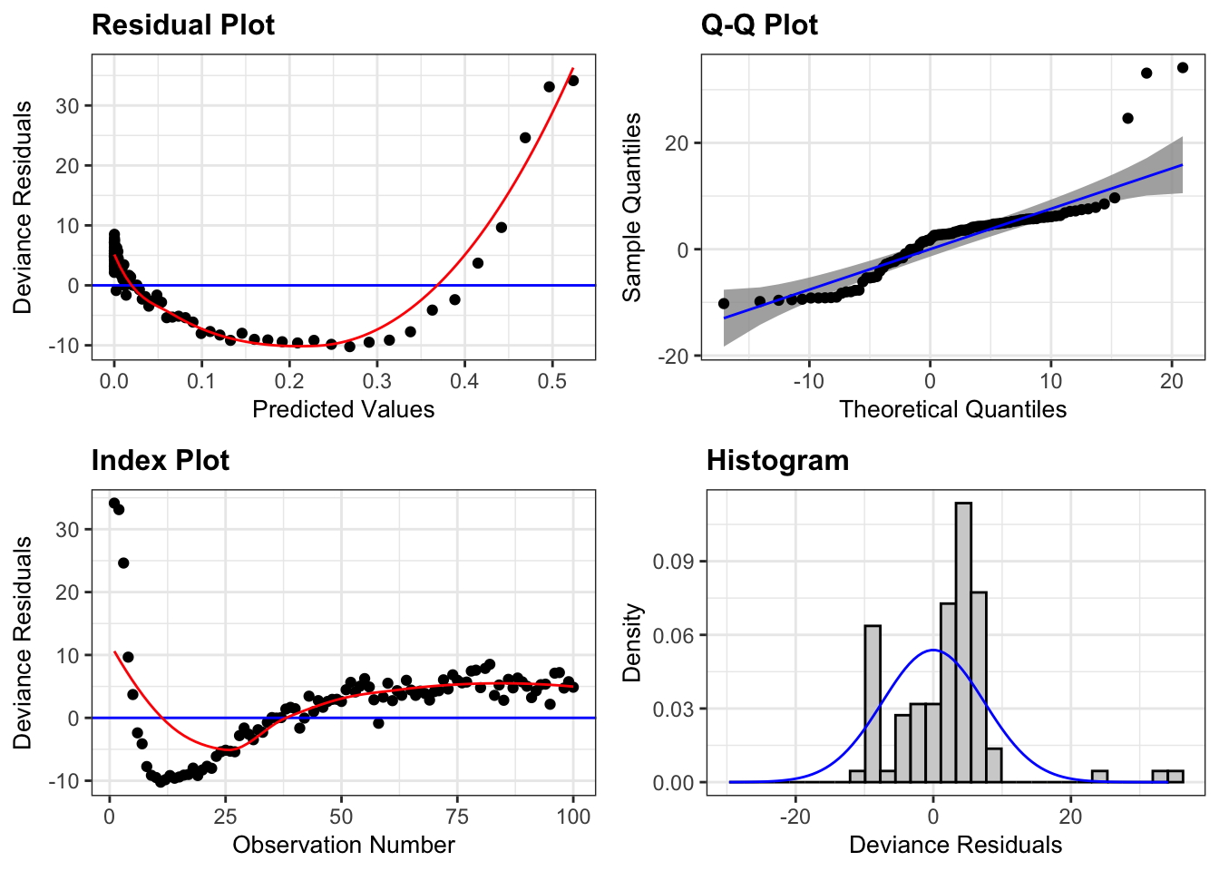
Let’s fit a logistic regression model to these data. We’ll start with just using distance,
`geom_smooth()` using formula = 'y ~ x'
`geom_smooth()` using formula = 'y ~ x'
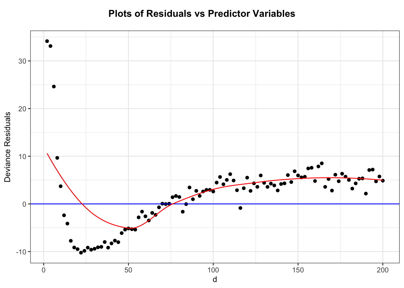
This plot shows clear violation of model assumptions. If we take a look at residuals vs distance plot we can see why.
ggResidpanel::resid_xpanel(m_d, smoother =TRUE)
`geom_smooth()` using formula = 'y ~ x'
We could also plot the estimated
Thus, it is clear we need an improved model, i.e. we need to include a higher order term for distance. Let’s try the terms the original authors used.
m_d2 <-glm(cbind(y, n - y) ~ d +I(d^2), data = simulated_putts,family ="binomial")
In a generalized linear model, e.g. logistic regression, we can use a drop-in-deviance test to evaluate the strength of evidence for terms in a model. If we look at sequential tests, the default in anova() then we can just keep terms
Like the authors, all of these terms are significant. We could have even tried more terms, but let’s stick with these.
summary(m_d2)
Call:
glm(formula = cbind(y, n - y) ~ d + I(d^2), family = "binomial",
    data = simulated_putts)

Coefficients:
              Estimate Std. Error z value Pr(>|z|)
(Intercept)  1.081e+00  2.849e-02   37.93   <2e-16 ***
d           -1.099e-01  1.301e-03  -84.48   <2e-16 ***
I(d^2)       4.276e-04  6.972e-06   61.34   <2e-16 ***
---
Signif. codes:  0 '***' 0.001 '**' 0.01 '*' 0.05 '.' 0.1 ' ' 1

(Dispersion parameter for binomial family taken to be 1)

    Null deviance: 24784.1  on 99  degrees of freedom
Residual deviance:  2864.9  on 97  degrees of freedom
AIC: 3329.9

Number of Fisher Scoring iterations: 5
While the anova() output shows sequential tests, i.e. adding one term at a time, this analysis suggests that, after including the logarithm of distance, we perhaps didn’t need any of the other distances. So let’s rearrange the terms.
m_d3 <-glm(cbind(y, n - y) ~log(d) + d +I(d^2) +I(d^3) +I(d^4), data = simulated_putts,family ="binomial")anova(m_d3)
Call:
glm(formula = cbind(y, n - y) ~ log(d) + d + I(d^2) + I(d^3) +
    I(d^4), family = "binomial", data = simulated_putts)

Coefficients:
              Estimate Std. Error z value Pr(>|z|)
(Intercept)  7.621e+00  2.642e-01  28.840  < 2e-16 ***
log(d)      -3.855e+00  1.899e-01 -20.304  < 2e-16 ***
d            1.344e-01  2.069e-02   6.497 8.22e-11 ***
I(d^2)      -1.313e-03  3.068e-04  -4.279 1.88e-05 ***
I(d^3)       6.912e-06  2.106e-06   3.282  0.00103 **
I(d^4)      -1.420e-08  5.099e-09  -2.785  0.00536 **
---
Signif. codes:  0 '***' 0.001 '**' 0.01 '*' 0.05 '.' 0.1 ' ' 1

(Dispersion parameter for binomial family taken to be 1)

    Null deviance: 24784.07  on 99  degrees of freedom
Residual deviance:   140.93  on 94  degrees of freedom
AIC: 611.94

Number of Fisher Scoring iterations: 4
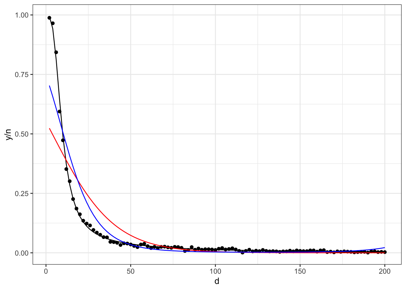
ggplot(simulated_putts, aes(x = d, y = y / n)) +geom_point() +geom_line(aes(y =predict(m_d3, type ="response"))) +geom_line(aes(y =predict(m_d, type ="response")), col='red') +geom_line(aes(y =predict(m_d2, type ="response")), col='blue')
Fearing, Douglas, Jason Acimovic, and Stephen C Graves. 2011. “How to Catch a Tiger: Understanding Putting Performance on the PGA Tour.”Journal of Quantitative Analysis in Sports 7 (1).