Warning: package 'purrr' was built under R version 4.4.1
── Attaching core tidyverse packages ──────────────────────── tidyverse 2.0.0 ──
✔ dplyr     1.1.4.9000     ✔ readr     2.1.5
✔ forcats   1.0.0          ✔ stringr   1.5.1
✔ ggplot2   3.5.1          ✔ tibble    3.2.1
✔ lubridate 1.9.3          ✔ tidyr     1.3.1
✔ purrr     1.0.4
── Conflicts ────────────────────────────────────────── tidyverse_conflicts() ──
✖ dplyr::filter() masks stats::filter()
✖ dplyr::lag()    masks stats::lag()
ℹ Use the conflicted package (<http://conflicted.r-lib.org/>) to force all conflicts to become errors
library("ggResidpanel")
4.1 Model
Let \(Y_i\in\{0,1,2,\ldots\}\) be a count (typically over some amount of time or some amount of space) with associated explanatory variables \(X_{i,1}, \ldots, X_{i,p}\).
Then a Poisson regression model is \[
Y_i \stackrel{ind}{\sim} Po(\lambda_i)
\] and \[
\log(\lambda_i)
= \beta_0 + \beta_1 X_{i,1} + \beta_2 X_{i,2} + \cdots +\beta_p X_{i,p}
\]
As a reminder, \(E[Y_i] = Var[Y_i] = \lambda_i\) and thus the variance of the observations increases as the mean increases.
4.2 Interpretation
When all explanatory variables are zero, then \[
E[Y_i|X_{i,1} = 0, \ldots,X_{i,p} = 0] = \lambda_i = e^{\beta_0}
\]
thus \(\beta_0\) determines the expected response when all explanatory variables are zero.
More generally, \[
E[Y_i|X_{i,1}=x_1, \ldots,X_{i,p}=x_p]
= e^{\beta_0+\beta_1x_1+\cdots+\beta_px_p}.
\]
If \(X_{i,1}\) increases by one unit, we have \[
E[Y_i|X_{i,1}=x_1+1, \ldots,X_{i,p}=x_p]
= e^{\beta_0+\beta_1(x_1+1)+\cdots+\beta_px_p}
= e^{\beta_0+\beta_1x_1+\cdots+\beta_px_p}e^{\beta_1}
\]
Thus \(e^{\beta_p}\) is the multiplicative effect on the mean response for a one unit increase in the associated explanatory variable when holding all other explanatory variables constant.
Rather than reporting the multiplicate effect, it is common to report the percentage increase (or decrease). To obtain the percentage increase, we calculate \[100(e^{\beta_p} - 1).\]
4.3 Assumptions
Observations are independent
Observations have a Poisson distribution
Count
Variance is equal to the mean
Relationship between expected response relationship and the explanatory variables is given by the model
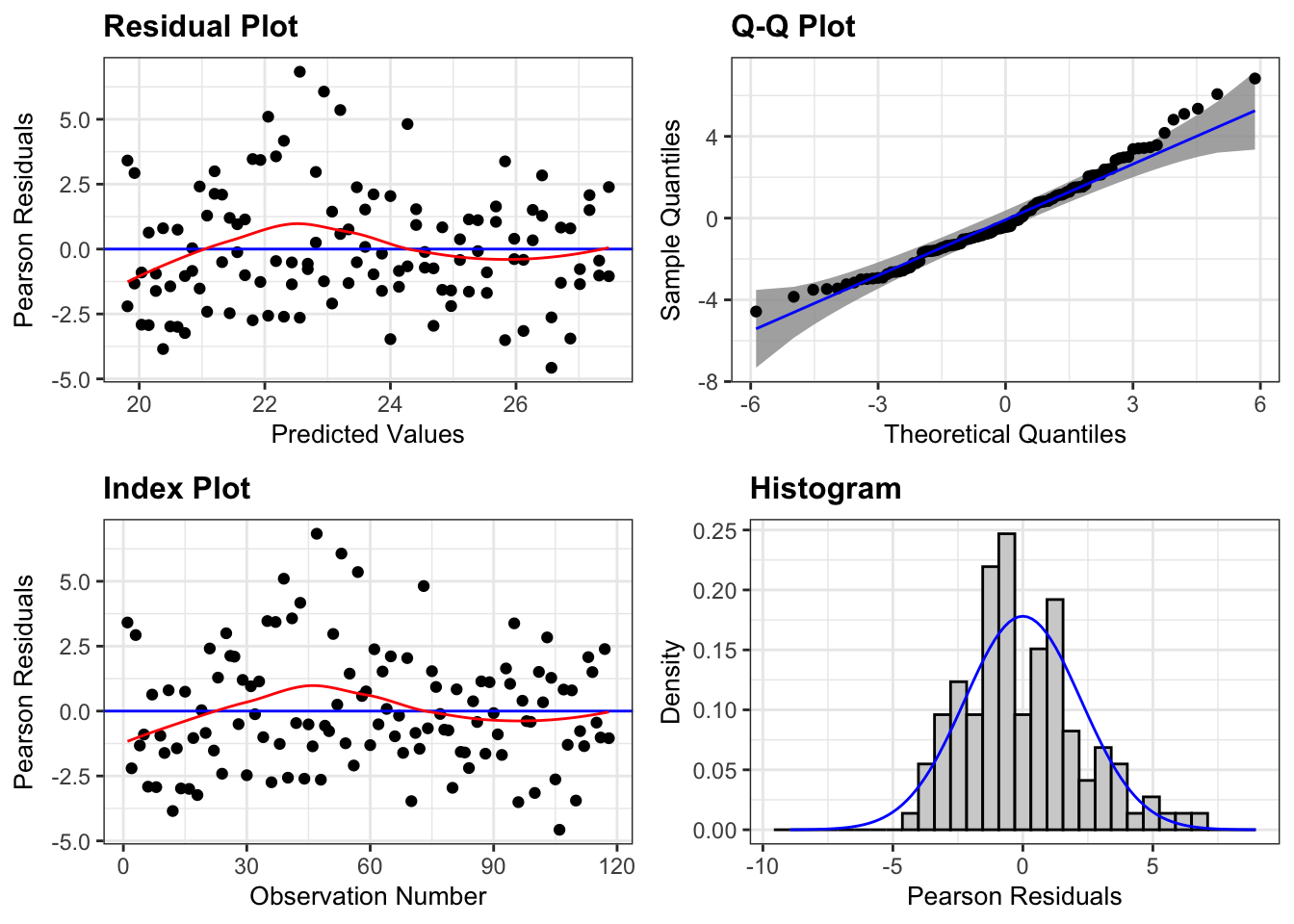
4.4 Diagnostics
Diagnostics in Poisson regression models is much harder because we don’t have the same idea of residuals as we had for linear regression models. We can compute some residuals: \[
r_i = Y_i - \hat{Y}_i = Y_i - \lambda_i
\] but these residuals each have a different variance. Thus, we need to standardize by calculating the Pearson residual\[
r_i^P = \frac{Y_i - \lambda_i}{\sqrt{\lambda_i}}
\]
Rows: 59 Columns: 4
── Column specification ────────────────────────────────────────────────────────
Delimiter: ","
chr (4): NO., DATE, SITE, RESULT

ℹ Use `spec()` to retrieve the full column specification for this data.
ℹ Specify the column types or set `show_col_types = FALSE` to quiet this message.
head(superbowl_scores)
# A tibble: 6 × 6
  NO.   DATE       SITE                          team    points  year
  <chr> <date>     <chr>                         <chr>    <dbl> <dbl>
1 I     1967-01-15 Los Angeles Memorial Coliseum winning     35  1967
2 I     1967-01-15 Los Angeles Memorial Coliseum losing      10  1967
3 II    1968-01-14 Orange Bowl (Miami)           winning     33  1968
4 II    1968-01-14 Orange Bowl (Miami)           losing      14  1968
5 III   1969-01-12 Orange Bowl (Miami)           winning     16  1969
6 III   1969-01-12 Orange Bowl (Miami)           losing       7  1969
summary(superbowl_scores)
     NO.                 DATE                SITE               team
 Length:118         Min.   :1967-01-15   Length:118         Length:118
 Class :character   1st Qu.:1981-04-26   Class :character   Class :character
 Mode  :character   Median :1996-01-28   Mode  :character   Mode  :character
                    Mean   :1996-01-28
                    3rd Qu.:2010-11-07
                    Max.   :2025-02-09
     points           year
 Min.   : 3.00   Min.   :1967
 1st Qu.:16.00   1st Qu.:1981
 Median :22.50   Median :1996
 Mean   :23.44   Mean   :1996
 3rd Qu.:31.00   3rd Qu.:2011
 Max.   :55.00   Max.   :2025
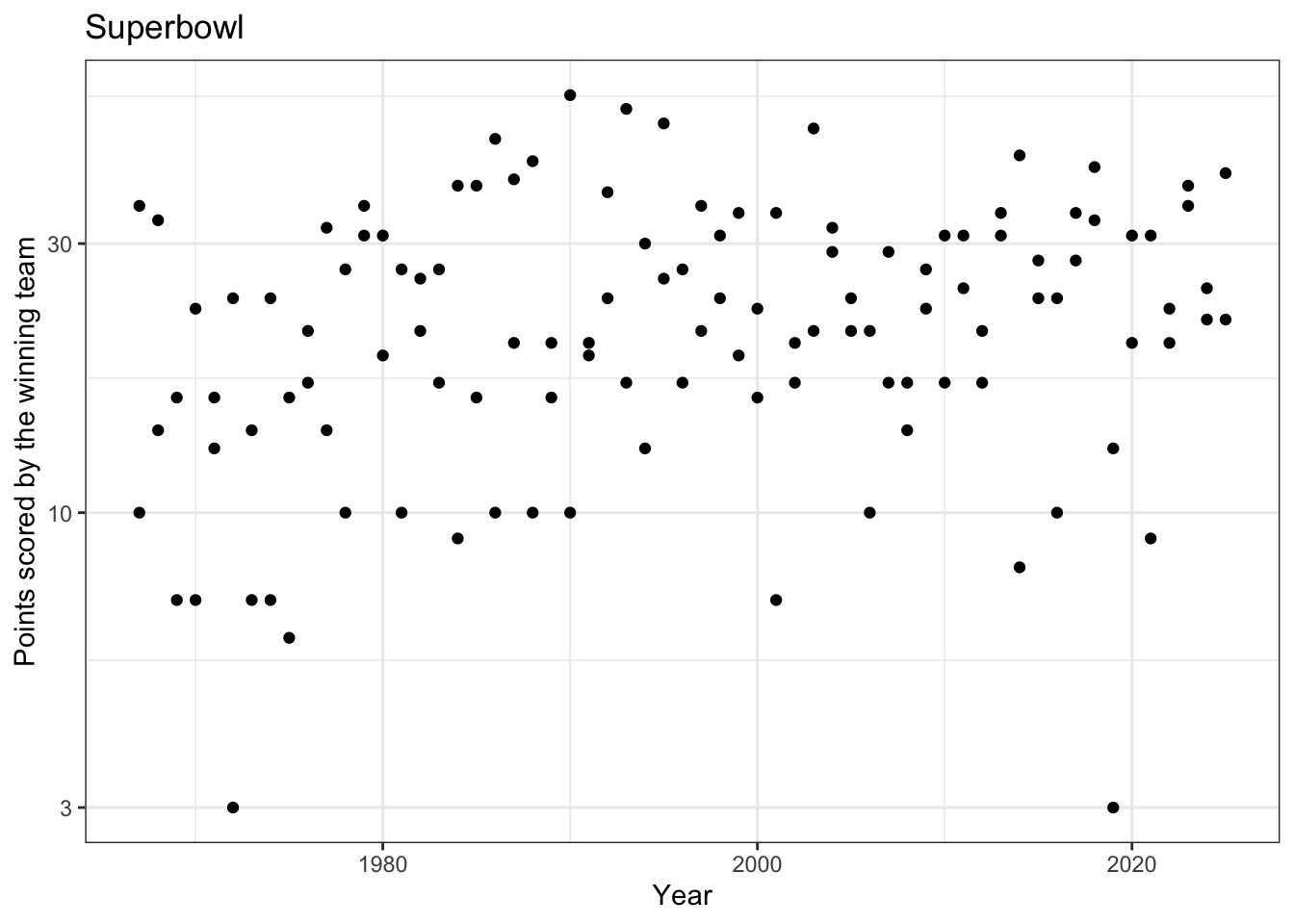
4.5.1 Points over time
Scientific question: How has the number of points changed over time?
ggplot(superbowl_scores,aes(x = year, y = points)) +geom_point() +scale_y_log10() +# Consistent with Poisson regressionlabs(x ="Year",y ='Points scored by the winning team',title ='Superbowl' )
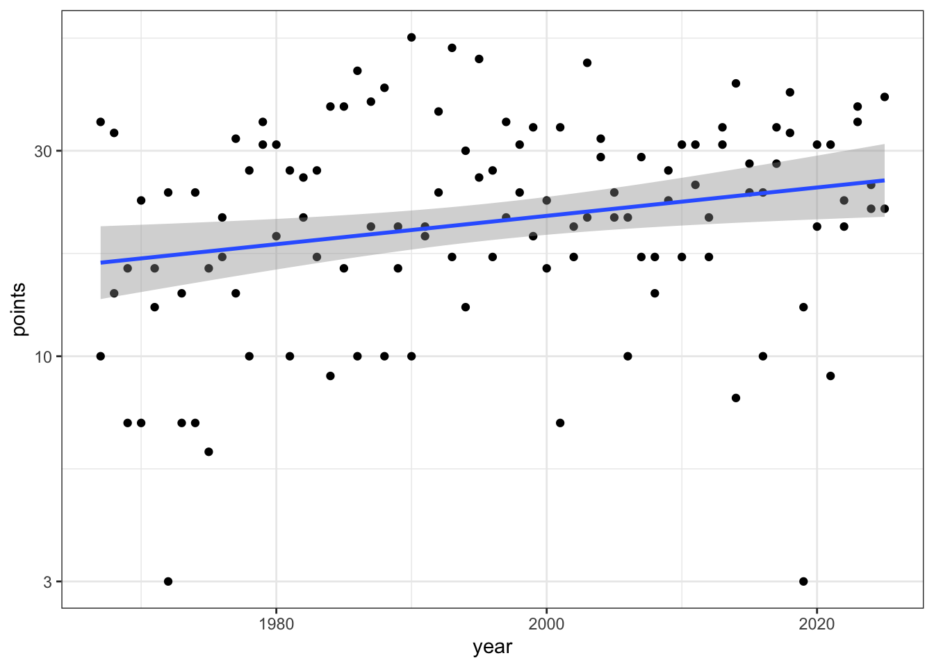
Let’s fit a Poisson regression model using points as the response variable and year as the explanatory variable.
# Poisson regressionm <-glm(points ~ year, # use glm()data = superbowl_scores, family ="poisson") # Poisson regressionm
Call:  glm(formula = points ~ year, family = "poisson", data = superbowl_scores)

Coefficients:
(Intercept)         year
  -8.105722     0.005639

Degrees of Freedom: 117 Total (i.e. Null);  116 Residual
Null Deviance:      620.5
Residual Deviance: 595.1    AIC: 1174
`geom_smooth()` using formula = 'y ~ x'
`geom_smooth()` using formula = 'y ~ x'
summary(m)
Call:
glm(formula = points ~ year, family = "poisson", data = superbowl_scores)

Coefficients:
             Estimate Std. Error z value Pr(>|z|)
(Intercept) -8.105722   2.236668  -3.624  0.00029 ***
year         0.005639   0.001120   5.037 4.74e-07 ***
---
Signif. codes:  0 '***' 0.001 '**' 0.01 '*' 0.05 '.' 0.1 ' ' 1

(Dispersion parameter for poisson family taken to be 1)

    Null deviance: 620.54  on 117  degrees of freedom
Residual deviance: 595.10  on 116  degrees of freedom
AIC: 1173.8

Number of Fisher Scoring iterations: 4
# Estimates and confidence intervalscbind(coef(m), confint(m)) |>exp() |>round(3)
# Calculate the percentage increaseperinc <-100*(exp(c(coef(m)[2], confint(m)[2,])) -1)
Waiting for profiling to be done...
perinc |>round(2)
  year  2.5 % 97.5 %
  0.57   0.35   0.79
Interpretation
We ran a Poisson regression using number of points each team scored as the response variable and year as the explanatory variable. According to the model, the expected points in year 0 for the winning team is 0 with a 95% confidence interval of (0, 0). The percentage increase in points by the winning team per year is 0.57% (0.35%, 0.79%).
The Poisson regression does indicate some overdispersion, i.e. that the variance is larger than the mean. A quick check looks at the residual deviance relative to its degrees of freedom. If there is no overdispersion, then the residual deviance should have a chi-squared distribution with the indicated degrees of freedom. Thus, if the residual deviance is very large compared to its degrees of freedom we likely have overdispersion.
# p-value for an overdispersion test1-pchisq(m$deviance, m$df.residual)
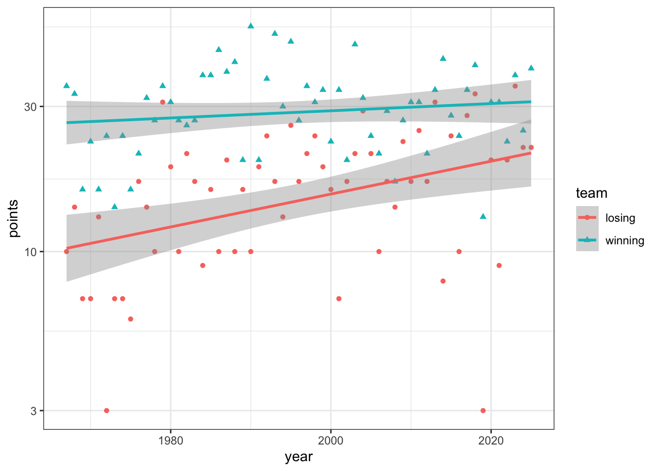
We ran a Poisson regression with number of points scored and winning/losing team as the explanatory variable. According to the model, the expected points for the losing team is 17 with a 95% confidence interval of (16, 18). The percentage increase in points by the winning team compared to the losing team is 81% (68%, 96%).
4.5.3 Points after adjusting for year
m <-glm(points ~ team + year, data = superbowl_scores,family ="poisson")summary(m)
Call:
glm(formula = points ~ team + year, family = "poisson", data = superbowl_scores)

Coefficients:
             Estimate Std. Error z value Pr(>|z|)
(Intercept) -8.447123   2.236836  -3.776 0.000159 ***
teamwinning  0.595443   0.039726  14.989  < 2e-16 ***
year         0.005639   0.001120   5.037 4.74e-07 ***
---
Signif. codes:  0 '***' 0.001 '**' 0.01 '*' 0.05 '.' 0.1 ' ' 1

(Dispersion parameter for poisson family taken to be 1)

    Null deviance: 620.54  on 117  degrees of freedom
Residual deviance: 360.38  on 115  degrees of freedom
AIC: 941.09

Number of Fisher Scoring iterations: 4
We ran a Poisson regression with number of points scored as the response variable and winning/losing team and year as the explanatory variables. According to the model, the expected points for the losing team in year 0 is 0 with a 95% confidence interval of (0, 0). After adjusting for year, the percentage increase in expected points by the winning team compared to the losing team is 81.4% (67.8%, 96.1%). After adjusting for winning versus losing team, the percentage increase in expected points by the both teams per year is 0.6% (0.3%, 0.8%).
4.5.4 Interaction
m <-glm(points ~ team * year, # Note the * rather than +data = superbowl_scores,family ="poisson")summary(m)
Call:
glm(formula = points ~ team * year, family = "poisson", data = superbowl_scores)

Coefficients:
                   Estimate Std. Error z value Pr(>|z|)
(Intercept)      -21.105150   3.791641  -5.566 2.60e-08 ***
teamwinning       20.149723   4.700361   4.287 1.81e-05 ***
year               0.011973   0.001896   6.314 2.72e-10 ***
teamwinning:year  -0.009787   0.002352  -4.161 3.17e-05 ***
---
Signif. codes:  0 '***' 0.001 '**' 0.01 '*' 0.05 '.' 0.1 ' ' 1

(Dispersion parameter for poisson family taken to be 1)

    Null deviance: 620.54  on 117  degrees of freedom
Residual deviance: 342.99  on 114  degrees of freedom
AIC: 925.7

Number of Fisher Scoring iterations: 4