6 Margin of Victory

library("tidyverse"); theme_set(theme_bw())

Warning: package 'purrr' was built under R version 4.4.1

── Attaching core tidyverse packages ──────────────────────── tidyverse 2.0.0 ──
✔ dplyr     1.1.4.9000     ✔ readr     2.1.5     
✔ forcats   1.0.0          ✔ stringr   1.5.1     
✔ ggplot2   3.5.1          ✔ tibble    3.2.1     
✔ lubridate 1.9.3          ✔ tidyr     1.3.1     
✔ purrr     1.0.4          
── Conflicts ────────────────────────────────────────── tidyverse_conflicts() ──
✖ dplyr::filter() masks stats::filter()
✖ dplyr::lag()    masks stats::lag()
ℹ Use the conflicted package (<http://conflicted.r-lib.org/>) to force all conflicts to become errors

library("ggResidpanel")

A simple example of margin-of-victory data is this fictitious collection of 4 teams that have played 5 games.

d <- tribble(
  ~home, ~away, ~home_score, ~away_score, 
      1,     2,          21,           7,
      2,     3,          13,          14,
      4,     1,           3,          28,
      3,     4,          31,           0,
      1,     3,          42,          10
) |>
  mutate(
    margin = home_score - away_score
  )

For the analysis that follows, we will construct a model matrix $X$ where $X_{g,t} = 1$ if team $t$ is the home team in game $g$,
$X_{g,t} = -1$ if team $t$ is the away team in game $g$, $X_{g,t} = 0$ otherwise.

construct_model_matrix <- function(d) {
  n_games <- nrow(d)
  n_teams <- length(unique(c(d$home, d$away)))
  
  m <- matrix(0, 
              nrow = n_games, 
              ncol = n_teams)
  
  for (g in 1:n_games) {
    m[g, d$home[g]] <-  1
    m[g, d$away[g]] <- -1
  }
  
  return(m)
}

X <- construct_model_matrix(d)
X

     [,1] [,2] [,3] [,4]
[1,]    1   -1    0    0
[2,]    0    1   -1    0
[3,]   -1    0    0    1
[4,]    0    0    1   -1
[5,]    1    0   -1    0

6.1 Model

A model for the margin of victory is

\[M_g = \eta + \theta_{H[g]} - \theta_{A[g]} + \epsilon_g\]

where, for game $g$,

$M_g$ is the margin of victory,
$H[g]$ is the ID for the home team,
$A[g]$ is the ID for the away team,
$\epsilon_g$ is a random error.

This error arises because if two teams play each other repeatedly we would expect that the score in their games would be random around the expected margin of victory.

The parameters are

$\eta$ is the home field advantage
$\theta_t$ is the strength of team $t$.

The expected margin of victory when team $H$ is at home playing against team $A$ is

\[E[M] = \eta + \theta_{H} - \theta_{A}.\]

6.1.1 Identifiability

In this model, when two teams play each other, the margin of victory is expected to be the home field advantage $\eta$ plus the difference in strengths between the two teams $\theta_H - \theta_A$. Thus, the individual $\theta$s are not identifiable, but only there difference is. Another way to state this is that we could add a constant to all of the team strengths and it would not change the distribution of the margin of victory since \[(\theta_H + c) - (\theta_A + c) = \theta_H - \theta_A.\] Even though the individual $\theta$ are not identifiable, the differences are.

Identifiable

Parameters (or functions of parameters) within a model are said to be identifiable if they can theoretically be estimated with an infinite amount of (the right kind of) data. That is, as you collect more and more data, the uncertainty in the parameter decreases to zero.

6.1.2 Regression

If we assume $\epsilon_i \stackrel{ind}{\sim} N(0,\sigma^2)$, then this is a linear regression model. To see how it is a linear regression model, we use the model matrix above and construct the following model

\[M_i = \eta + \theta_1 X_{i,1} + \theta_2 X_{i,2} + \theta_3 X_{i,3} + \theta_4 X_{i,4} + \epsilon_i, \quad \epsilon_i \stackrel{ind}{\sim} N(0,\sigma^2)\].

Thus, we can estimate the parameters in this model using linear regression.

m <- lm(d$margin ~ X) # intercept (home-field advantage) is included automatically

summary(m)


Call:
lm(formula = d$margin ~ X)

Residuals:
     1      2      3      4      5 
-7.917 -7.917  2.639  2.639 10.556 

Coefficients: (1 not defined because of singularities)
            Estimate Std. Error t value Pr(>|t|)
(Intercept)    7.389      7.464   0.990    0.503
X1            35.028     12.656   2.768    0.221
X2            20.500     15.833   1.295    0.419
X3            20.972     12.656   1.657    0.346
X4                NA         NA      NA       NA

Residual standard error: 15.83 on 1 degrees of freedom
Multiple R-squared:  0.8904,    Adjusted R-squared:  0.5615 
F-statistic: 2.707 on 3 and 1 DF,  p-value: 0.4137

From this model, we can obtain individual values for $\theta$. The estimated values are

coef(m)

(Intercept)          X1          X2          X3          X4 
   7.388889   35.027778   20.500000   20.972222          NA

With these data, the estimated home field advantage is $= 7.3888889. The estimated ability for the teams are

coef(m)[-1]

      X1       X2       X3       X4 
35.02778 20.50000 20.97222       NA

The fourth team has an estimated value of $\theta_4 = NA$, i.e. not available. The reason for this is the identifiability issue above.

Here, the $NA$ can be replaced by 0.

team_ability <- coef(m)[-1]
team_ability[4] <- 0
team_ability

      X1       X2       X3       X4 
35.02778 20.50000 20.97222  0.00000

Using these team ability estimates, we can compute the expected point difference between the teams. For example, on a neutral court, the expected point difference between team 1 and team 2 is

team_ability[1] - team_ability[2] # expected point difference on a neutral court

      X1 
14.52778

So Team 1 is expected to beat Team 2 by 15 points.

6.1.3 Prediction

In addition to the expected point difference, you can use this model to predict the probability that one team beats the other team. In order to perform this prediction, we need to know the variability around the expected point spread. We can extract this information from the regression model. The estimated residual standard deviation is

summary(m)$sigma

[1] 15.83333

Prediction in a regression model utilizes a $t$ distribution with degrees of freedom equal to the number of observations minus the number of teams. This is given in the R output.

summary(m)$df[2]

[1] 1

Thus to calculate the probability that Team 1 beats Team 2 on a neutral court we calculate \[P\left(T_v < \frac{\theta_1 - \theta_2}{\hat\sigma}\right).\] In R code, we have

pt( (team_ability[1] - team_ability[2]) / summary(m)$sigma, summary(m)$df[2] )

       X1 
0.7363208

6.1.4 Transitivity

One drawback of these types of models is that the model is transitive, but this may not reflect reality. The transitivity property in this model is \[\theta_A > \theta_B \quad\&\quad \theta_B > \theta_C \,\implies\, \theta_A > \theta_C.\] In words, this means that if Team A is better than Team B and Team B is better than Team C, then Team A must be better than Team C. This precludes the possibility that Team C could match up well against Team A.

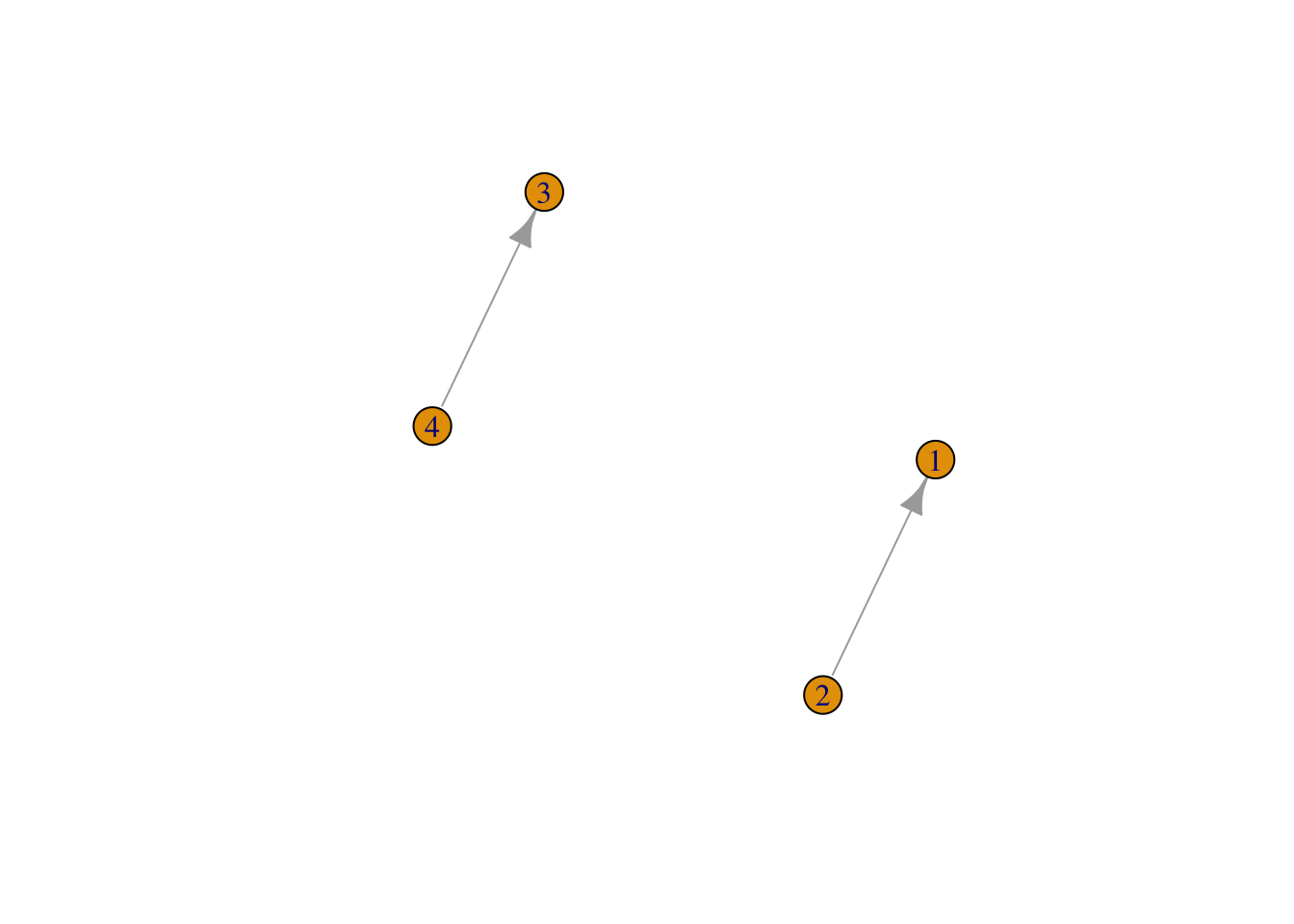
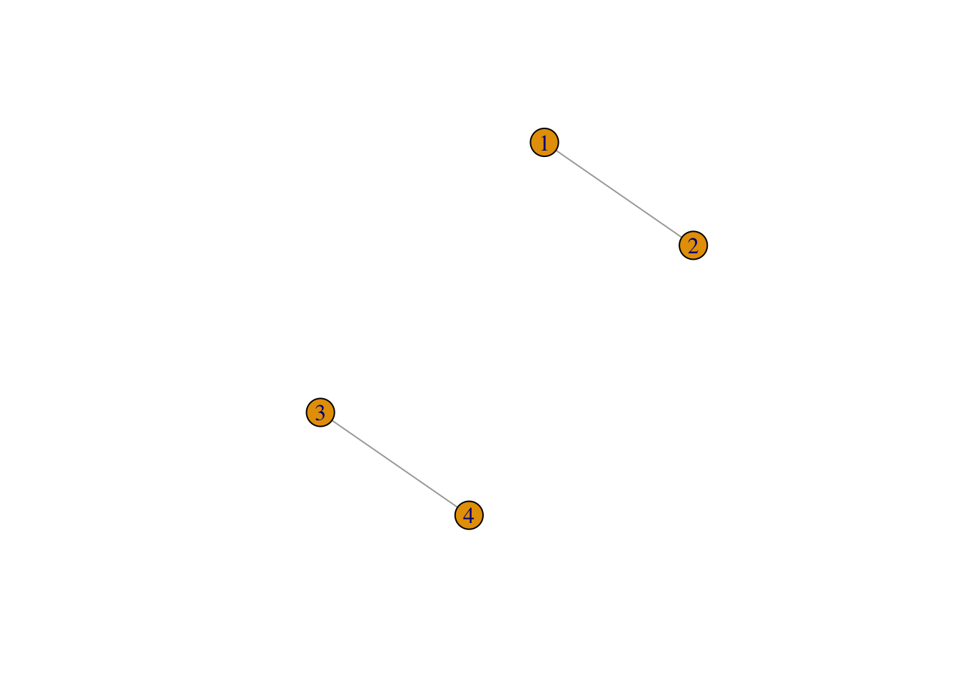
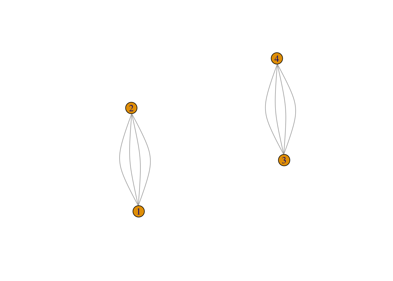
As an example, consider the following set of teams and games.

d2 <- tribble(
  ~home, ~away, ~margin, 
      1,     2,     100,   
      2,     3,      90, 
      3,     1,      95,
  
      2,     1,    -100,   
      3,     2,     -90, 
      1,     3,     -95
)

If these were data for basketball games, we would expect that Team 1 has a high probability of beating Team 2, Team 2 has a high probability of beating Team 3, and Team 3 has a high probability of beating Team 1.

Fitting the model above and estimating the probstrengths tells a different story.

X2 <- construct_model_matrix(d2)

m2 <- lm(d2$margin ~ X2)
summary(m2)


Call:
lm(formula = d2$margin ~ X2)

Residuals:
  1   2   3   4   5   6 
 95  95  95 -95 -95 -95 

Coefficients: (1 not defined because of singularities)
              Estimate Std. Error t value Pr(>|t|)
(Intercept)  3.599e-15  5.485e+01   0.000    1.000
X21          2.220e-15  7.757e+01   0.000    1.000
X22         -5.000e+00  7.757e+01  -0.064    0.953
X23                 NA         NA      NA       NA

Residual standard error: 134.4 on 3 degrees of freedom
Multiple R-squared:  0.001843,  Adjusted R-squared:  -0.6636 
F-statistic: 0.00277 on 2 and 3 DF,  p-value: 0.9972

We can already see issues here since none of the coefficients are significantly different from zero.

# Calculate team strengths
team_ability <- coef(m2)[-1]
team_ability[3] <- 0
team_ability

          X21           X22           X23 
 2.220446e-15 -5.000000e+00  0.000000e+00

# Calculate probstrengths
pt( (team_ability[1] - team_ability[2]) / summary(m2)$sigma, summary(m2)$df[2])

      X21 
0.5136747

pt( (team_ability[1] - team_ability[3]) / summary(m2)$sigma, summary(m2)$df[2])

X21 
0.5

pt( (team_ability[2] - team_ability[3]) / summary(m2)$sigma, summary(m2)$df[2])

      X22 
0.4863253

6.1.5 Estimability

Consider this set of teams and games

d3 <- tribble(
  ~home, ~away, ~margin, 
      1,     2,      10,   
      3,     4,       9
)

From these data, we cannot determine how good teams 1-2 and compared to teams 3-4. Even if with a lot more data we may not be able to estimate the model parameters.

d4 <- tribble(
  ~home, ~away, ~margin, 
      1,     2,      10,   
      3,     4,       9, 
      1,     2,       5,   
      3,     4,      13, 
      1,     2,       1,   
      3,     4,      -3, 
      1,     2,       2,   
      3,     4,      -6 
)

If we try to actually fit this model,

X4 <- construct_model_matrix(d4)
m4 <- lm(d4$margin ~ X4)
summary(m4)


Call:
lm(formula = d4$margin ~ X4)

Residuals:
   Min     1Q Median     3Q    Max 
-9.250 -4.188 -1.000  5.562  9.750 

Coefficients: (3 not defined because of singularities)
            Estimate Std. Error t value Pr(>|t|)
(Intercept)    3.250      3.546   0.917    0.395
X41            1.250      5.015   0.249    0.811
X42               NA         NA      NA       NA
X43               NA         NA      NA       NA
X44               NA         NA      NA       NA

Residual standard error: 7.092 on 6 degrees of freedom
Multiple R-squared:  0.01025,   Adjusted R-squared:  -0.1547 
F-statistic: 0.06214 on 1 and 6 DF,  p-value: 0.8115

While previously we had only 1 line with NAs, we now have 3 lines with NAs.

Estimability

Parameters are said to be estimable with a certain said of data if the parameters can be estimated with that data. Thus parameters may be identifiable but not estimable while parameters that are not identifiable are never estimable.

6.1.5.1 Graphs

In these models, the graph of team contests is helpful.

library("igraph")


Attaching package: 'igraph'

The following objects are masked from 'package:lubridate':

    %--%, union

The following objects are masked from 'package:dplyr':

    as_data_frame, groups, union

The following objects are masked from 'package:purrr':

    compose, simplify

The following object is masked from 'package:tidyr':

    crossing

The following object is masked from 'package:tibble':

    as_data_frame

The following objects are masked from 'package:stats':

    decompose, spectrum

The following object is masked from 'package:base':

    union

plot(graph_from_data_frame(d3[,c(2,1)]))          # arrows point away -> home

plot(graph_from_data_frame(d3, directed = FALSE))

plot(graph_from_data_frame(d4, directed = FALSE))

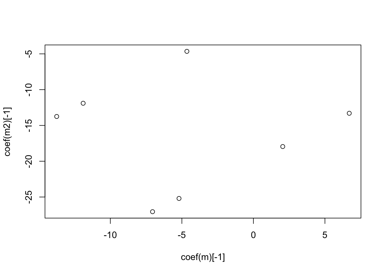
Parameters (or functions of parameters) may also be weakly estimable. Consider these data

d_conf <- tribble(
  ~home, ~away, ~margin, 
      1,     2,      10, # Conference 1  
      3,     4,       9, 
      2,     3,      -2,
      1,     4,     -20,
      3,     1,       4,
      4,     2,      16,
      5,     6,      10, # Conference 2
      7,     8,       9, 
      6,     7,      -2,
      5,     8,     -20,
      7,     5,       4,
      8,     6,      16,
      1,     5,      10 # Inter-conference Game
)

plot(graph_from_data_frame(d_conf[, c(2,1)]))

Predict the outcome for two teams

# Predict the outcome for 3 vs 7
Xconf <- construct_model_matrix(d_conf)
m <- lm(d_conf$margin ~ Xconf)
summary(m)


Call:
lm(formula = d_conf$margin ~ Xconf)

Residuals:
         1          2          3          4          5          6          7 
 4.850e+00  1.035e+01  3.800e+00 -1.140e+01 -6.550e+00 -1.050e+00  4.850e+00 
         8          9         10         11         12         13 
 1.035e+01  3.800e+00 -1.140e+01 -6.550e+00 -1.050e+00 -2.092e-15 

Coefficients: (1 not defined because of singularities)
            Estimate Std. Error t value Pr(>|t|)
(Intercept)    3.300      3.572   0.924    0.398
Xconf1        -5.200     14.837  -0.350    0.740
Xconf2        -7.050     16.371  -0.431    0.685
Xconf3         2.050     16.851   0.122    0.908
Xconf4         6.700     16.371   0.409    0.699
Xconf5       -11.900      8.185  -1.454    0.206
Xconf6       -13.750      7.988  -1.721    0.146
Xconf7        -4.650      8.185  -0.568    0.595
Xconf8            NA         NA      NA       NA

Residual standard error: 11.3 on 5 degrees of freedom
Multiple R-squared:  0.6168,    Adjusted R-squared:  0.08026 
F-statistic:  1.15 on 7 and 5 DF,  p-value: 0.4547

# Expected point difference (neutral court)
(exp_diff <- coef(m)[4] - coef(m)[8])

Xconf3 
   6.7

# Probability of winning (neutral court)
pt( exp_diff / summary(m)$sigma, df = summary(m)$df[2])

   Xconf3 
0.7105335

Now let’s change the result for the intraconference game and see what happens.

d_conf2 <- d_conf
d_conf2$margin[nrow(d_conf2)]        # old score

[1] 10

d_conf2$margin[nrow(d_conf2)] <- -10 # new score

# Predict the outcome for 3 vs 7
Xconf2 <- construct_model_matrix(d_conf2)
m2 <- lm(d_conf2$margin ~ Xconf2)
summary(m2)


Call:
lm(formula = d_conf2$margin ~ Xconf2)

Residuals:
         1          2          3          4          5          6          7 
 4.850e+00  1.035e+01  3.800e+00 -1.140e+01 -6.550e+00 -1.050e+00  4.850e+00 
         8          9         10         11         12         13 
 1.035e+01  3.800e+00 -1.140e+01 -6.550e+00 -1.050e+00 -3.795e-15 

Coefficients: (1 not defined because of singularities)
            Estimate Std. Error t value Pr(>|t|)
(Intercept)    3.300      3.572   0.924    0.398
Xconf21      -25.200     14.837  -1.698    0.150
Xconf22      -27.050     16.371  -1.652    0.159
Xconf23      -17.950     16.851  -1.065    0.335
Xconf24      -13.300     16.371  -0.812    0.453
Xconf25      -11.900      8.185  -1.454    0.206
Xconf26      -13.750      7.988  -1.721    0.146
Xconf27       -4.650      8.185  -0.568    0.595
Xconf28           NA         NA      NA       NA

Residual standard error: 11.3 on 5 degrees of freedom
Multiple R-squared:  0.6394,    Adjusted R-squared:  0.1346 
F-statistic: 1.267 on 7 and 5 DF,  p-value: 0.4111

# Expected point difference (neutral court)
(exp_diff2 <- coef(m2)[4] - coef(m2)[8])

Xconf23 
  -13.3

# Probability of winning (neutral court)
pt( exp_diff2 / summary(m2)$sigma, df = summary(m2)$df[2])

  Xconf23 
0.1460273

Inter-conference play determines amount of ``strength’’ allocated to the conference.

plot(coef(m)[-1], coef(m2)[-1])

6.2 Rating Systems

6.2.1 Sagarin Ratings

An example of publish margin of victory model estimates are Sagarin Ratings. There is an R package that may be able to scrape Sagarin ratings. Argh, these have stopped being updated in 2023.

6.2.2 Ken Pomeroy

I believe Ken Pomeroy’s ratings are based on these margin-of-victory models.

6.3 Examples

6.3.1 Iowa High School Football

6.3.2 International Handball

handball2024 <- read_csv("data/Handball_W_InternationalResults.csv",
                     col_types = cols(
                       ScoreA = col_double(),
                       ScoreB = col_double(),
                       year = col_integer(),
                       Date = col_date(),
                       .default = col_character()
                     )) |>
  filter(year == 2024) |>
  mutate(
    margin = ScoreA - ScoreB
  )

# plot(graph_from_data_frame(handball[,c("TeamA","TeamB")]), directed = FALSE)

library("networkD3")

p <- simpleNetwork(handball2024, 
                   height="100px", width="100px",        
        Source = "TeamA",                 # column number of source
        Target = "TeamB",                 # column number of target
        linkDistance = 10,          # distance between node. Increase this value to have more space between nodes
        charge = -900,                # numeric value indicating either the strength of the node repulsion (negative value) or attraction (positive value)
        fontSize = 14,               # size of the node names
        fontFamily = "serif",       # font og node names
        linkColour = "#666",        # colour of edges, MUST be a common colour for the whole graph
        nodeColour = "#69b3a2",     # colour of nodes, MUST be a common colour for the whole graph
        opacity = 0.9,              # opacity of nodes. 0=transparent. 1=no transparency
        zoom = T                    # Can you zoom on the figure?
        )

p

separated_countries <- c("Romania", "Bosnia and Herzegovina", "Greece", "Croatia")

handball2024b <- handball2024 |>
  filter(!( TeamA %in% separated_countries | TeamB %in% separated_countries) )

# Convert team names into factors
teams <- data.frame(
  names = c(handball2024b$TeamA, handball2024b$TeamB) |>
    unique() |>
    sort() |>
    factor()
) 

X_h <- handball2024b |>
  rename(
    home = TeamA,
    away = TeamB
  ) |>
  mutate(
    home = factor(home, levels = teams$names),
    away = factor(away, levels = teams$names)
  ) |>
  construct_model_matrix()

dim(X_h) # n_games x n_teams

[1] 160  44

m <- lm(handball2024b$margin ~ X_h - 1) # remove the home field advantage
summary(m)$sigma

[1] 5.900357

teams$strength <- coef(m)
teams$strength[nrow(teams)] <- 0
teams$strength <- teams$strength - mean(teams$strength)

teams$names <- factor(teams$names, levels = teams$names[order(teams$strength)])

ggplot(teams, 
       aes(
         x = strength,
         y = names
       )) +
  geom_bar(stat = "identity")

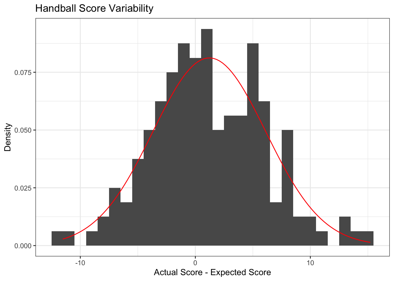
The distribution of scores around the expected score.

ggplot() +
  geom_histogram(
    aes(
      x = m$residuals,
        y = after_stat(density)
    ), # Get frequency rather than count
    binwidth = 1,
  ) +
  stat_function(
    fun  = dnorm, 
    args = list(
      mean = mean(m$residuals),
      sd   = sd(m$residuals)
    ), 
    color = "red"
  ) +
  labs(
    x = 'Actual Score - Expected Score',
    y = 'Density',
    title = 'Handball Score Variability'
  )

I was expecting these residuals to be centered at 0, but I fit a model that did not include an intercept (since there was no clear home field). Perhaps an intercept was needed?

# Refit model with intercept
m <- lm(handball2024b$margin ~ X_h) 
summary(m)$coefficients[1,]

   Estimate  Std. Error     t value    Pr(>|t|) 
1.281715708 0.466134486 2.749669350 0.006921771

It appears the intercept is significant. Taking a look at the data, there appears to be a Venue listed and this Venue would provide information about a possible home-field advantage. The analysis here would likely need to be a bit more complex as the home-field advantage should only be listed when a team is actually playing at home.

handball2024b |> 
  select(TeamA, TeamB, Venue) |> 
  as.data.frame()

              TeamA           TeamB           Venue
1           Germany         Ukraine         Germany
2           Ukraine        Slovakia          Poland
3          Slovakia         Germany        Slovakia
4            Israel         Ukraine        Slovakia
5           Ukraine          Israel        Slovakia
6           Germany        Slovakia         Germany
7            Israel        Slovakia         Germany
8           Ukraine         Germany         Germany
9           Germany          Israel         Germany
10         Slovakia         Ukraine        Slovakia
11   Czech Republic         Finland  Czech Republic
12      Netherlands        Portugal     Netherlands
13          Finland     Netherlands         Finland
14         Portugal  Czech Republic        Portugal
15   Czech Republic     Netherlands  Czech Republic
16          Finland        Portugal         Finland
17      Netherlands  Czech Republic     Netherlands
18         Portugal         Finland        Portugal
19          Finland  Czech Republic         Finland
20         Portugal     Netherlands        Portugal
21      Netherlands         Finland     Netherlands
22   Czech Republic        Portugal  Czech Republic
23         Slovenia          Latvia        Slovenia
24           France           Italy          France
25           Latvia          France          Latvia
26            Italy        Slovenia           Italy
27         Slovenia          France        Slovenia
28           Latvia           Italy          Latvia
29           France        Slovenia          France
30            Italy          Latvia           Italy
31            Italy          France           Italy
32           Latvia        Slovenia          Latvia
33           France          Latvia          France
34         Slovenia           Italy        Slovenia
35  North Macedonia      Azerbaijan North Macedonia
36            Spain       Lithuania           Spain
37       Azerbaijan           Spain      Azerbaijan
38        Lithuania North Macedonia       Lithuania
39       Azerbaijan       Lithuania      Azerbaijan
40  North Macedonia           Spain North Macedonia
41        Lithuania      Azerbaijan       Lithuania
42            Spain North Macedonia           Spain
43       Azerbaijan North Macedonia      Azerbaijan
44        Lithuania           Spain       Lithuania
45            Spain      Azerbaijan           Spain
46  North Macedonia       Lithuania North Macedonia
47       Montenegro          Turkey      Montenegro
48           Serbia        Bulgaria          Serbia
49         Bulgaria      Montenegro        Bulgaria
50           Turkey          Serbia          Turkey
51         Bulgaria          Turkey        Bulgaria
52           Serbia      Montenegro          Serbia
53           Turkey        Bulgaria          Turkey
54       Montenegro          Serbia      Montenegro
55           Turkey      Montenegro          Turkey
56         Bulgaria          Serbia        Bulgaria
57       Montenegro        Bulgaria      Montenegro
58           Serbia          Turkey          Serbia
59          Iceland      Luxembourg         Iceland
60           Sweden   Faroe Islands          Sweden
61       Luxembourg          Sweden      Luxembourg
62    Faroe Islands         Iceland   Faroe Islands
63       Luxembourg   Faroe Islands      Luxembourg
64          Iceland          Sweden         Iceland
65           Sweden         Iceland          Sweden
66    Faroe Islands      Luxembourg   Faroe Islands
67       Luxembourg         Iceland      Luxembourg
68    Faroe Islands          Sweden   Faroe Islands
69           Sweden      Luxembourg          Sweden
70          Iceland   Faroe Islands         Iceland
71          Denmark          Kosovo         Denmark
72           Kosovo         Denmark          Kosovo
73           Poland         Denmark          Poland
74          Denmark          Poland         Denmark
75           Kosovo          Poland          Kosovo
76           Poland          Kosovo          Poland
77      Switzerland         Austria     Switzerland
78          Hungary          Norway         Hungary
79           Norway     Switzerland          Norway
80          Austria         Hungary         Austria
81          Hungary     Switzerland         Hungary
82           Norway         Austria          Norway
83      Switzerland         Hungary     Switzerland
84          Austria          Norway         Austria
85          Austria     Switzerland         Austria
86           Norway         Hungary          Norway
87      Switzerland          Norway     Switzerland
88          Hungary         Austria         Hungary
89         Cameroon           Congo          Angola
90           Angola         Senegal          Angola
91         Cameroon         Senegal          Angola
92            Congo          Angola          Angola
93          Senegal           Congo          Angola
94           Angola        Cameroon          Angola
95            China      Kazakhstan           Japan
96      South Korea           India           Japan
97            India           Japan           Japan
98      South Korea           China           Japan
99            Japan      Kazakhstan           Japan
100           China           India           Japan
101           China           Japan           Japan
102      Kazakhstan     South Korea           Japan
103      Kazakhstan           India           Japan
104           Japan     South Korea           Japan
105         Hungary   Great Britain         Hungary
106          Sweden           Japan         Hungary
107          Sweden         Hungary         Hungary
108           Japan   Great Britain         Hungary
109   Great Britain          Sweden         Hungary
110         Hungary           Japan         Hungary
111  Czech Republic           Spain           Spain
112     Netherlands       Argentina           Spain
113     Netherlands  Czech Republic           Spain
114       Argentina           Spain           Spain
115  Czech Republic       Argentina           Spain
116           Spain     Netherlands           Spain
117         Germany        Slovenia         Germany
118      Montenegro        Paraguay         Germany
119         Germany      Montenegro         Germany
120        Slovenia        Paraguay         Germany
121        Paraguay         Germany         Germany
122      Montenegro        Slovenia         Germany
123        Slovenia         Denmark          France
124         Germany     South Korea          France
125          Norway          Sweden          France
126     South Korea        Slovenia          France
127          Sweden         Germany          France
128         Denmark          Norway          France
129         Germany        Slovenia          France
130          Norway     South Korea          France
131          Sweden         Denmark          France
132     South Korea          Sweden          France
133         Germany         Denmark          France
134        Slovenia          Norway          France
135        Slovenia          Sweden          France
136          Norway         Germany          France
137         Denmark     South Korea          France
138     Netherlands          Angola          France
139           Spain          Brazil          France
140         Hungary          France          France
141          Brazil         Hungary          France
142          Angola           Spain          France
143          France     Netherlands          France
144     Netherlands           Spain          France
145         Hungary          Angola          France
146          France          Brazil          France
147     Netherlands          Brazil          France
148           Spain         Hungary          France
149          Angola          France          France
150         Hungary     Netherlands          France
151           Spain          France          France
152          Brazil          Angola          France
153         Denmark     Netherlands          France
154          France         Germany          France
155         Hungary          Sweden          France
156          Norway          Brazil          France
157          Sweden          France          France
158          Norway         Denmark          France
159         Denmark          Sweden          France
160          Norway          France          France

6.3.3 College Baseball 2024

baseball <- read.csv("data/college_baseball_2024.csv")

Let’s take a look at these data. (Really I got quite a way in the analysis and realized an issue, so now I’m back fixing up the data.)

str(baseball)

'data.frame':   123 obs. of  6 variables:
 $ Dates     : chr  "3/17/2023" "3/17/2023" "3/17/2023" "3/18/2023" ...
 $ Team_1    : chr  "Kansas State" "Texas Christian" "Texas Tech" "Baylor" ...
 $ Score_1   : int  8 13 8 8 9 3 8 7 12 7 ...
 $ Team_2    : chr  "Baylor" "Oklahoma" "Oklahoma State" "Kansas State" ...
 $ Score_2   : int  1 5 7 4 4 1 4 5 1 1 ...
 $ Home_Field: chr  "@Baylor" "@Oklahoma" "@Texas Tech" "@Baylor" ...

sort(unique(c(baseball$Team_1, baseball$Team_2)))

[1] "Baylor"          "Kansas"          "Kansas State"    "Oklahoma"       
[5] "Oklahoma State"  "Texas"           "Texas Christian" "Texas Tech"     
[9] "West Virginia"

sort(unique(baseball$Home_Field)) # there are neutral sites

 [1] "@Baylor"          "@Kansas"          "@Kansas State"    "@neutral"        
 [5] "@Oklahoma"        "@Oklahoma State"  "@Texas"           "@Texas Christian"
 [9] "@Texas Tech"      "@West Virginia"

# Compared to sports we have been looking at baseball scores are relatively low
# with most scores 10 or below
table(c(baseball$Score_1, baseball$Score_2))


 0  1  2  3  4  5  6  7  8  9 10 11 12 13 14 15 16 17 18 19 20 21 
 4 17 18 26 21 26 28 21 19 14 15  5  8  5  4  4  2  2  3  2  1  1

Let’s deal explicitly with neutral sites.

baseball2024 <- baseball |>
  
  # Create home/away teams and scores
  # for neutral sites, home/away will be arbitrary
  mutate(
    Home_Field = gsub("@", "", Home_Field),
    home_is_Team_1 =                        # this is used repeatedly below
      Home_Field == "neutral" | 
        Home_Field == Team_1,  
    
    # Set the teams
    home = ifelse(home_is_Team_1, Team_1, Team_2),
    away = ifelse(home_is_Team_1, Team_2, Team_1),
    
    # Set the scores
    home_score = ifelse(home_is_Team_1, Score_1, Score_2),
    away_score = ifelse(home_is_Team_1, Score_2, Score_1),
    
    margin = home_score - away_score,
    
    Date = as.Date(Dates, format = "%m/%d/%Y")
  ) |>
  select(Date, Home_Field, home, away, home_score, away_score, margin)

Let’s first check the graph connectedness.

p <- simpleNetwork(baseball2024, 
                   height="100px", width="100px",        
        Source = "away",                 # column number of source
        Target = "home",                 # column number of target
        linkDistance = 10,          # distance between node. Increase this value to have more space between nodes
        charge = -900,                # numeric value indicating either the strength of the node repulsion (negative value) or attraction (positive value)
        fontSize = 14,               # size of the node names
        fontFamily = "serif",       # font og node names
        linkColour = "#666",        # colour of edges, MUST be a common colour for the whole graph
        nodeColour = "#69b3a2",     # colour of nodes, MUST be a common colour for the whole graph
        opacity = 0.9,              # opacity of nodes. 0=transparent. 1=no transparency
        zoom = T                    # Can you zoom on the figure?
        )

p

Let’s build our model for margin of victory depending on team strength and include home-field advantage when it is relevant.

To do so, we will create an additional column in the X matrix that includes a home-field advantage only when playing on a home-field, i.e. not at a neutral site. Then, when we run the regression, we will not include an intercept.

# Construct factors for teams
teams <- data.frame(
  names = c(baseball2024$home, baseball2024$away) |>
    unique() |>
    sort() |>
    factor()
)

baseball2024 <- baseball2024 |>
  mutate(
    home = factor(home, levels = teams$names),
    away = factor(away, levels = teams$names)
  )

X_baseball <- 
  cbind(
    1 * !(baseball2024$Home_Field == "neutral"),
    construct_model_matrix(baseball2024)
  )

colnames(X_baseball) <- c("home-field advantage", as.character(teams$names))

rowSums(X_baseball) # home_field advantage has a 1 and neutral is 0

  [1] 1 1 1 1 1 1 1 1 1 1 1 1 1 1 1 1 1 1 1 1 1 1 1 1 1 1 1 1 1 1 1 1 1 1 1 1 1
 [38] 1 1 1 1 1 1 1 1 1 1 1 1 1 1 1 1 1 1 1 1 1 1 1 1 1 1 1 1 1 1 1 1 1 1 1 1 1
 [75] 1 1 1 1 1 1 1 1 1 1 1 1 1 1 1 1 1 1 1 1 1 1 1 1 1 1 1 1 1 1 1 1 1 1 1 0 0
[112] 0 0 0 0 0 0 0 0 0 0 0 0

colSums(X_baseball) # difference in number of home - away games

home-field advantage               Baylor               Kansas 
                 109                    0                   -1 
        Kansas State             Oklahoma       Oklahoma State 
                   0                   -2                    3 
               Texas      Texas Christian           Texas Tech 
                  -2                    4                    0 
       West Virginia 
                  -2

head(X_baseball)

     home-field advantage Baylor Kansas Kansas State Oklahoma Oklahoma State
[1,]                    1      1      0           -1        0              0
[2,]                    1      0      0            0        1              0
[3,]                    1      0      0            0        0             -1
[4,]                    1      1      0           -1        0              0
[5,]                    1      0      0            0        0             -1
[6,]                    1      0      0            0        1              0
     Texas Texas Christian Texas Tech West Virginia
[1,]     0               0          0             0
[2,]     0              -1          0             0
[3,]     0               0          1             0
[4,]     0               0          0             0
[5,]     0               0          1             0
[6,]     0              -1          0             0

m <- lm(baseball2024$margin ~ X_baseball - 1) # remove intercept
summary(m)$sigma

[1] 5.403159

# Home field advantage
coef(m)[1]

X_baseballhome-field advantage 
                      1.399588

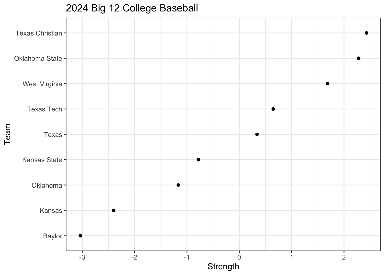
# Team strengths
strength <- coef(m)[-1]
strength[length(strength)] <- 0

teams <- teams |>
  mutate(
    strength = strength - mean(strength),
    names    = factor(names, 
                      levels = names[order(strength)])
  ) |>
  arrange(desc(strength))

ggplot(teams,
       aes(
         x = strength,
         y = names 
       )) +
  geom_point() +
  labs(
    x = "Strength",
    y = "Team",
    title = "2024 Big 12 College Baseball"
  )

One aspect of these data that have not been addressed is the bias due to the way the 9th inning works in baseball. In the bottom of the 9th inning, the home team immediately wins if they are ever ahead of the away team. This could happen sometime during the 9th inning or even before the bottom of the 9th inning occurs. The bias that results is likely a underestimate of the home field advantage because the home team scores less points than they could have.

6.4 R packages

Are there any or do we really have to do all of this by hand?