7  Win-Loss Models

In this chapter, we investigate models when you only observe the binary outcome of the home team winning the game.

library("tidyverse"); theme_set(theme_bw())
Warning: package 'purrr' was built under R version 4.4.1
── Attaching core tidyverse packages ──────────────────────── tidyverse 2.0.0 ──
✔ dplyr     1.1.4.9000     ✔ readr     2.1.5     
✔ forcats   1.0.0          ✔ stringr   1.5.1     
✔ ggplot2   3.5.1          ✔ tibble    3.2.1     
✔ lubridate 1.9.3          ✔ tidyr     1.3.1     
✔ purrr     1.0.4          
── Conflicts ────────────────────────────────────────── tidyverse_conflicts() ──
✖ dplyr::filter() masks stats::filter()
✖ dplyr::lag()    masks stats::lag()
ℹ Use the conflicted package (<http://conflicted.r-lib.org/>) to force all conflicts to become errors
library("DT")
library("BradleyTerry2")

A simple example of margin-of-victory data is this fictitious collection of 4 teams that have played 5 games.

d <- tribble(
  ~home, ~away, ~home_score, ~away_score, 
      1,     2,          21,           7,
      2,     3,          13,          14,
      4,     1,           3,          28,
      3,     4,          31,           0,
      1,     3,          42,          10
) |>
  mutate(
    home_win = home_score > away_score # binary indicator of who won
  )

For the analysis that follows, we will construct a model matrix \(X\) where \(X_{g,t} = 1\) if team \(t\) is the home team in game \(g\),
\(X_{g,t} = -1\) if team \(t\) is the away team in game \(g\), \(X_{g,t} = 0\) otherwise.

construct_model_matrix <- function(d, homeCol = "home", awayCol = "away") {
  n_games <- nrow(d)
  n_teams <- length(unique(unlist(d[, homeCol], d[, awayCol])))
  
  m <- matrix(0, 
              nrow = n_games, 
              ncol = n_teams)
  
  for (g in 1:n_games) {
    m[g, as.numeric(d[g, homeCol])] <-  1
    m[g, as.numeric(d[g, awayCol])] <- -1
  }
  
  return(m)
}

X <- construct_model_matrix(d)
X
     [,1] [,2] [,3] [,4]
[1,]    1   -1    0    0
[2,]    0    1   -1    0
[3,]   -1    0    0    1
[4,]    0    0    1   -1
[5,]    1    0   -1    0

7.1 Model

A model for the indicator of who won is

\[H_g \stackrel{ind}{\sim} Ber(\pi_g)\]

where

  • \(H_g\) is the indicator that the home team won game \(g\) and
  • \(\pi_g\) is the probability the home team would win game \(g\).

The probability of winning the game is then related to the team strength using the typical logit function.

\[\mbox{logit}(\pi_g) = \log \left( \frac{\pi_g}{1-\pi_g} \right) = \eta_g = \eta + \theta_{H[g]} - \theta_{A[g]}\]

where, for game \(g\),

  • \(H[g]\) is the ID for the home team, and
  • \(A[g]\) is the ID for the away team.

The parameters are

  • \(\eta\) is the home field advantage
  • \(\theta_t\) is the strength of team \(t\).

The probability of team H winning at home against team A is.

\[\pi_g = \mbox{expit}(\eta_g) = \left\{ 1 + \exp[-\eta_g] \right\}^{-1} = \left\{ 1 + \exp[-(\eta + \theta_{H} - \theta_{A})] \right\}^{-1}\]

expit <- function(eta) {
  1 / (1 + exp(-eta))
}

7.1.1 Identifiability

Similar to the margin-of-victory models, the individual \(\theta\)s are not identifiable, but only their difference is.

7.1.2 Graph connectednss

Just like the margin of victory models we will also have identifiability issues if the graph isn’t connected. If the graph is sparsely connected, as happens with conference play, then games that connect parts of the graph will have an outsized influence on the overall estimate of team strength.

7.1.3 Separation

An issue that exists in these models for binary outcome that doesn’t exist for the margin-of-victory models is the issue of separation.

Separation

A complete separation in a win-loss model occurs when one team has either won or lost all of their games.

If a team has won all of their games, then it is impossible to determine how good that team is. Thus their team strength can be arbitrarily large.

m <- glm(d$home_win ~ X, family = binomial(link = "logit")) 
Warning: glm.fit: fitted probabilities numerically 0 or 1 occurred

The warning in this output is an indication that separation has occurred.

summary(m)

Call:
glm(formula = d$home_win ~ X, family = binomial(link = "logit"))

Coefficients: (1 not defined because of singularities)
              Estimate Std. Error z value Pr(>|z|)
(Intercept)      7.429  72844.703       0        1
X1              32.606 125856.238       0        1
X2             -14.266 153887.408       0        1
X3              16.709  95064.223       0        1
X4                  NA         NA      NA       NA

(Dispersion parameter for binomial family taken to be 1)

    Null deviance: 6.7301e+00  on 4  degrees of freedom
Residual deviance: 3.5615e-10  on 1  degrees of freedom
AIC: 8

Number of Fisher Scoring iterations: 23

The large standard errors are another indication that separation has occurred. Of course, it is best practice to make sure that every team has won and lost at least one game before you get to the step of fitting the model.

Separation can also be observed if the home team wins every game. In this situation, the home advantage parameter can be arbitrarily large.

Other separation situations can occur. For example, imagine that there are two conferences and, in every inter-conference game, one conference wins all the games. In this situation, we have no information about how much better one conference is than the other.

Separation is typical problem in logistic regression models, but particularly a problem in the types of models we are using for win-loss data.

7.1.4 Transivity

Similar to margin-of-victory models, this win-loss model is transitive: if Team A is better than Team B and Team B is better than Team C then Team A is better than Team C. That is, there is no information about specific matchups.

7.2 Rating Systems

Anybody know of any purely win-loss ratings systems? Perhaps one of the tennis rating systems:

7.3 Examples

7.3.1 Iowa High School Football

football <- read.csv("data/Iowa_High_School_Football_4A_Game_Scores_2018.csv") |>
  filter(Playoffs == 0) |> # Not playoffs
  mutate(
    home_win = HomeScore > AwayScore
  )

Let’s take a look at the graph

library("networkD3")

Attaching package: 'networkD3'
The following object is masked from 'package:DT':

    JS
p <- simpleNetwork(football, 
                   height="100px", width="100px",        
        Source = "AwayTeam",               
        Target = "HomeTeam",            
        linkDistance = 10,          # distance between node. Increase this value to have more space between nodes
        charge = -900,                # numeric value indicating either the strength of the node repulsion (negative value) or attraction (positive value)
        fontSize = 14,               # size of the node names
        fontFamily = "serif",       # font og node names
        linkColour = "#666",        # colour of edges, MUST be a common colour for the whole graph
        nodeColour = "#69b3a2",     # colour of nodes, MUST be a common colour for the whole graph
        opacity = 0.9,              # opacity of nodes. 0=transparent. 1=no transparency
        zoom = T                    # Can you zoom on the figure?
        )

p

Overall this graph looks reasonably connected.

# Proportion home wins
football |> summarize(p = mean(home_win))
          p
1 0.5284091

So we don’t have to worry about identifiability of the home-field advantage parameter.

# Team Win-Loss
football |>
  tidyr::pivot_longer(
    cols = c(`HomeTeam`, `AwayTeam`),
    names_to = "Location",
    values_to = "Team") |>
  group_by(Team) |>
  summarize(
    n_games = n(),
    wins    = sum( 
      (home_win & Location == "HomeTeam") |
      (!home_win & Location == "AwayTeam") ),
    loses   = n_games - wins,
    p       = wins/n_games
  ) |>
  arrange(desc(p)) |>
  datatable(
    filter = "top"
  )

With these data, we have many teams that either have all wins or all loses. These data are not appropriate for these models.

7.3.2 International Handball

handball2024 <- read_csv("data/Handball_W_InternationalResults.csv",
                     col_types = cols(
                       ScoreA = col_double(),
                       ScoreB = col_double(),
                       year = col_integer(),
                       Date = col_date(),
                       .default = col_character()
                     )) |>
  filter(year == 2024,
         !(TeamA %in% c("Romania", 
                        "Bosnia and Herzegovina", 
                        "Greece", 
                        "Croatia"))) |>
  mutate(
    margin = ScoreA - ScoreB,
    A_win  = margin > 0
  )

I didn’t bother calculating statistics here because due to the small number of games each team played, there will definitely be some teams that have 0 wins and some that have 0 loses.

7.3.3 Waterpolo

waterpolo <- read.csv("data/waterpolo_Men.csv") |>
  mutate(TeamA_win = Winner == TeamA) # Create binary win variable
waterpolo |>
  tidyr::pivot_longer(
    cols = c("TeamA", "TeamB"),
    names_to = "AorB",
    values_to = "Team"
  ) |>
  group_by(Team) |>
  summarize(
    n    = n(),
    wins = sum(
      (TeamA_win & AorB == "TeamA") |
        (!TeamA_win & AorB == "TeamB")
      ),
    loses = n - wins,
    p     = wins / n
  ) |>
  arrange(desc(p)) |>
  datatable(
    filter = "top"
  )

7.3.4 Tennis

tennis <- read.csv("data/tennis.csv") |>
  mutate(
    Date = as.Date(Date)
  ) |>
  # Select only 2019 games
  filter(Date > as.Date("2018-12-31")) |>
  select(Winner, Loser) 
tennis_win_loss <- tennis |>
  tidyr::pivot_longer(
    cols = c("Winner", "Loser"),
    names_to = "Win",
    values_to = "Player"
  ) |>
  group_by(Player) |>
  summarize(
    n    = n(),
    wins = sum(Win == "Winner"),
    loses = n - wins,
    p     = wins / n
  ) |>
  filter(n > 20) |>
  arrange(desc(p))

tennis_win_loss |>
  datatable(
    filter = "top"
  )

Limit the data to only individuals who have played at least 20 games. When we eliminate some games, the individuals remaining may have less than 20 games. The hope is that everybody has at least one win and one loss.

tennis_filtered <- tennis |>
  filter(
    Winner %in% tennis_win_loss$Player & 
      Loser %in% tennis_win_loss$Player
  )

tennis_filtered |>  
  tidyr::pivot_longer(
    cols = c("Winner", "Loser"),
    names_to = "Win",
    values_to = "Player"
  ) |>
  group_by(Player) |>
  summarize(
    n    = n(),
    wins = sum(Win == "Winner"),
    loses = n - wins,
    p     = wins / n
  ) |>
  # filter(n > 20) |>
  arrange(desc(p)) |>
  datatable(
    filter = "top"
  )

Everybody now has at least 1 win and 1 loss.

Check graph to make sure it is connected.

p <- simpleNetwork(tennis_filtered, 
                   height="100px", width="100px",        
        Source = "Winner",               
        Target = "Loser",            
        linkDistance = 10,          # distance between node. Increase this value to have more space between nodes
        charge = -900,                # numeric value indicating either the strength of the node repulsion (negative value) or attraction (positive value)
        fontSize = 14,               # size of the node names
        fontFamily = "serif",       # font og node names
        linkColour = "#666",        # colour of edges, MUST be a common colour for the whole graph
        nodeColour = "#69b3a2",     # colour of nodes, MUST be a common colour for the whole graph
        opacity = 0.9,              # opacity of nodes. 0=transparent. 1=no transparency
        zoom = T                    # Can you zoom on the figure?
        )

p

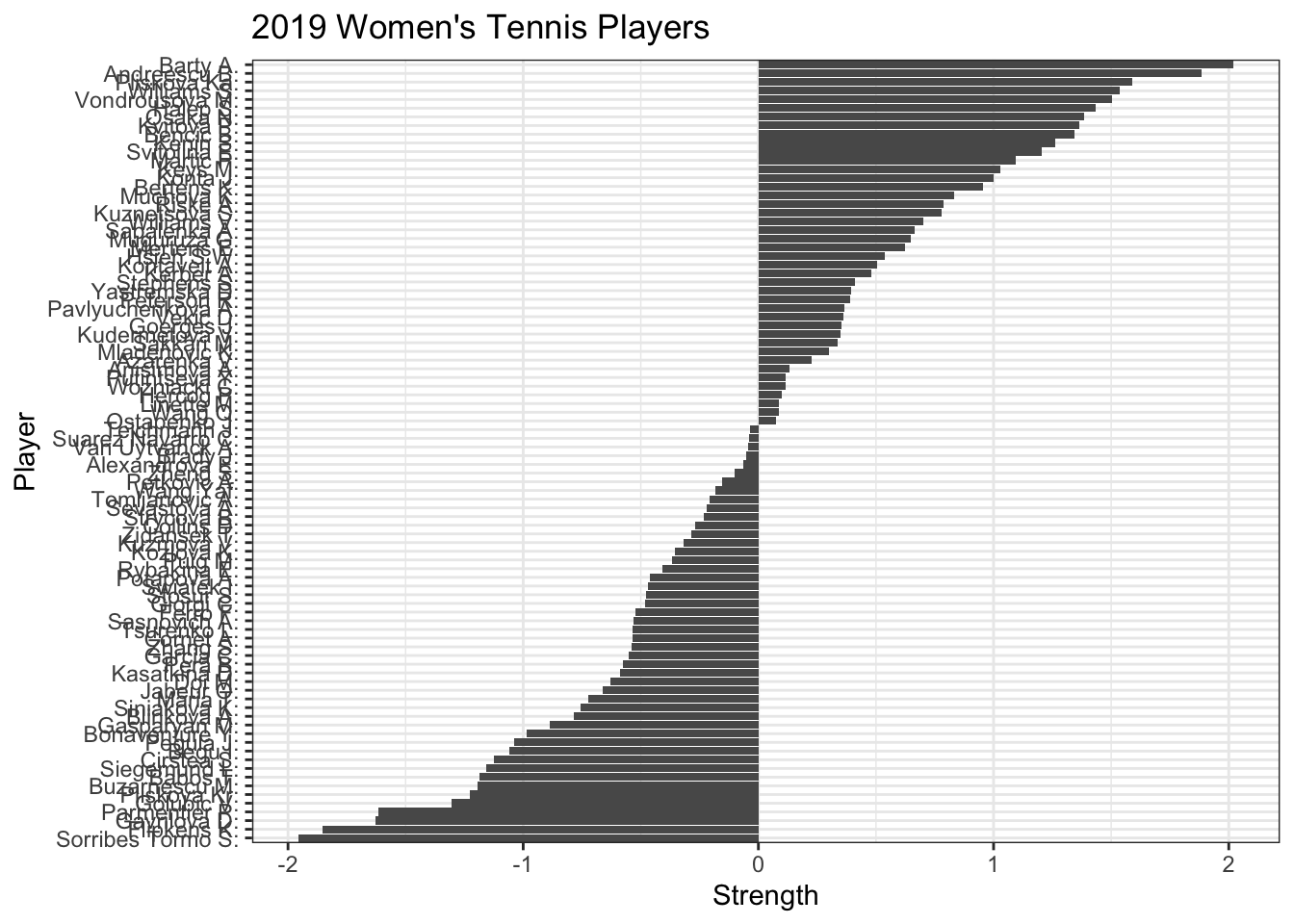
This graph looks complete and well connected. Perhaps this is unsurprising because the top tennis players play a lot of games against each other over the course of a year.

# Convert team names into factors
players <- data.frame(
  names = c(tennis_filtered$Winner, tennis_filtered$Loser) |>
    unique() |>
    sort() |>
    factor()
) 


tennis_filtered_factored <- tennis_filtered |>
  mutate(
    Winner = factor(Winner, levels = players$names),
    Loser  = factor(Loser,  levels = players$names)
  ) 

X_t <- tennis_filtered_factored |>
  construct_model_matrix("Winner", "Loser")

Check the model matrix

dim(X_t)                    # n_games x n_teams
[1] 1414   90
table(X_t)                  # make sure all entries are -1, 0, 1
X_t
    -1      0      1 
  1414 124432   1414 
all(rowSums(X_t) == 0)      # each row has one winner and one loser
[1] TRUE
all(rowSums(abs(X_t)) == 2) # ^
[1] TRUE
table(colSums(X_t))         # for each player, number of wins - number of loses

-17 -14 -13 -12 -10  -9  -8  -7  -6  -5  -4  -3  -2  -1   0   1   2   3   4   5 
  1   1   2   2   4   3   1   5  12   5   1   6   8   5   1   3   4   4   3   1 
  7   9  10  13  14  15  16  17  18  19  20  26  34 
  2   2   1   1   1   1   1   1   2   2   2   1   1 

Finally, we can fit our logistic regression model. For these data, we do not have a binary column that indicates the winner. Instead, we have a column that indicates the winner by name. Thus, we will need to create a binary column that indicates the first column (named Winner) is the winner.

# Fit logistic regression model
# since columns are Winner/Loser the result should always be TRUE,
# i.e. the first column won
m <- glm(rep(TRUE, nrow(X_t)) ~ X_t - 1, # no home field
         family = binomial(link = "logit")) 

tail(coef(m))         # includes last team as NA
     X_t85      X_t86      X_t87      X_t88      X_t89      X_t90 
 0.9837438  0.3987670  0.6788688 -0.2555386  0.1827746         NA 
tail(summary(m)$coef) # notice only 89 rows, but there are 90 teams
        Estimate Std. Error    z value    Pr(>|z|)
X_t84  1.8207497  0.6563103  2.7742211 0.005533406
X_t85  0.9837438  0.6277945  1.5669838 0.117118482
X_t86  0.3987670  0.6202366  0.6429272 0.520271365
X_t87  0.6788688  0.5733442  1.1840511 0.236392836
X_t88 -0.2555386  0.6176878 -0.4137019 0.679092435
X_t89  0.1827746  0.6000472  0.3046003 0.760670565
players$strength <- c(coef(m)[-length(coef(m))], 0)

player_strength <- players |>
  mutate(
    names = factor(names, 
                     levels = players$names[order(players$strength)]),
    strength = strength - mean(strength)
  ) |>
  arrange(desc(strength))

ggplot(player_strength,
       aes(
         x = strength,
         y = names
       )) +
  geom_bar(stat = "identity") +
  labs(
    x = 'Strength',
    y = 'Player',
    title = "2019 Women's Tennis Players"
  )

To calculate the probability that one player beats another we can calculate the difference in their strengths and then calculate the probability.

diff <- players$strength[players$names == "Barty A."] -
  players$strength[players$names == "Halep S."]

expit(diff)
[1] 0.642461

7.4 R packages

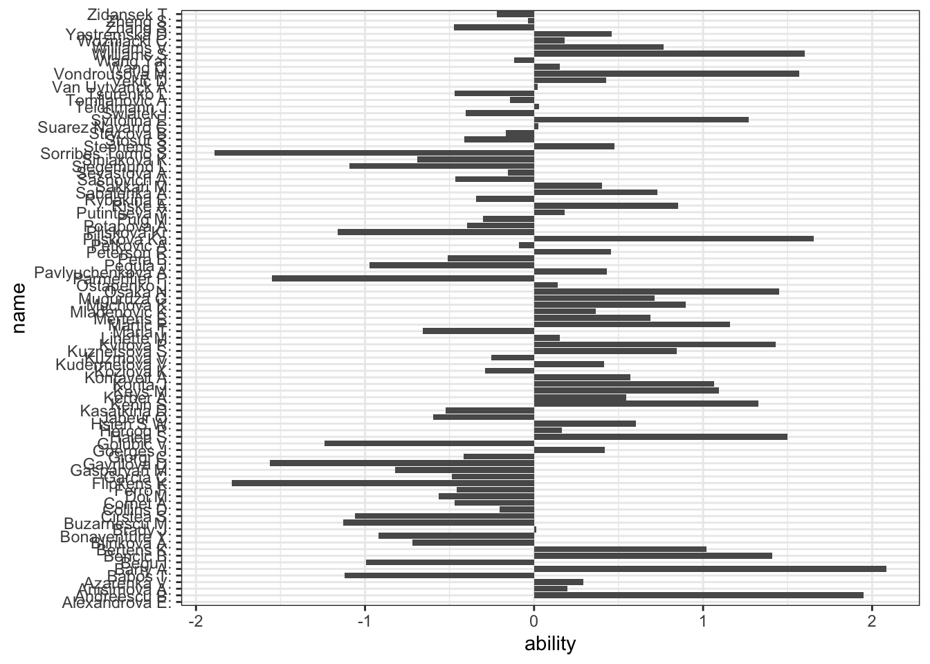
The models discussed in this chapter are often referred to as Bradley-Terry models after the 1952 Biometrika article written by Ralph Bradley and Milton Terry (Bradley and Terry 1952).

bt_m <- BradleyTerry2::BTm(player1 = Winner,
            player2 = Loser,
            data = tennis_filtered_factored)

summary(bt_m)

Call:
BradleyTerry2::BTm(player1 = Winner, player2 = Loser, data = tennis_filtered_factored)

Coefficients:
                    Estimate Std. Error z value Pr(>|z|)    
..Andreescu B.       1.94999    0.54629   3.570 0.000358 ***
..Anisimova A.       0.19720    0.57777   0.341 0.732870    
..Azarenka V.        0.29196    0.51307   0.569 0.569326    
..Babos T.          -1.12184    0.72819  -1.541 0.123417    
..Barty A.           2.08396    0.48064   4.336 1.45e-05 ***
..Begu I.           -0.99389    0.78898  -1.260 0.207775    
..Bencic B.          1.40985    0.44982   3.134 0.001723 ** 
..Bertens K.         1.02180    0.43455   2.351 0.018704 *  
..Blinkova A.       -0.72067    0.59866  -1.204 0.228665    
..Bonaventure Y.    -0.92131    0.65720  -1.402 0.160954    
..Brady J.           0.01215    0.53577   0.023 0.981914    
..Buzarnescu M.     -1.12972    0.58067  -1.946 0.051709 .  
..Cirstea S.        -1.05997    0.66069  -1.604 0.108639    
..Collins D.        -0.20407    0.53427  -0.382 0.702483    
..Cornet A.         -0.47105    0.54205  -0.869 0.384842    
..Doi M.            -0.56444    0.66026  -0.855 0.392617    
..Ferro F.          -0.45868    0.57552  -0.797 0.425463    
..Flipkens K.       -1.78898    0.67342  -2.657 0.007894 ** 
..Garcia C.         -0.48776    0.51046  -0.956 0.339307    
..Gasparyan M.      -0.82213    0.60911  -1.350 0.177107    
..Gavrilova D.      -1.56190    0.76995  -2.029 0.042501 *  
..Giorgi C.         -0.41830    0.57768  -0.724 0.468999    
..Goerges J.         0.42035    0.51729   0.813 0.416448    
..Golubic V.        -1.23970    0.66332  -1.869 0.061633 .  
..Halep S.           1.49790    0.46984   3.188 0.001432 ** 
..Hercog P.          0.16492    0.50337   0.328 0.743189    
..Hsieh S.W.         0.60157    0.47262   1.273 0.203071    
..Jabeur O.         -0.59852    0.54908  -1.090 0.275691    
..Kasatkina D.      -0.52272    0.55984  -0.934 0.350460    
..Kenin S.           1.32696    0.45803   2.897 0.003766 ** 
..Kerber A.          0.54516    0.47877   1.139 0.254838    
..Keys M.            1.09317    0.52465   2.084 0.037194 *  
..Konta J.           1.06582    0.48112   2.215 0.026742 *  
..Kontaveit A.       0.56882    0.51163   1.112 0.266233    
..Kozlova K.        -0.28802    0.60566  -0.476 0.634394    
..Kudermetova V.     0.41372    0.49361   0.838 0.401941    
..Kuzmova V.        -0.25375    0.51282  -0.495 0.620735    
..Kuznetsova S.      0.84488    0.58250   1.450 0.146940    
..Kvitova P.         1.42855    0.47270   3.022 0.002510 ** 
..Linette M.         0.15431    0.54488   0.283 0.777028    
..Maria T.          -0.65721    0.66608  -0.987 0.323798    
..Martic P.          1.15813    0.47007   2.464 0.013751 *  
..Mertens E.         0.69051    0.46513   1.485 0.137668    
..Mladenovic K.      0.36512    0.48121   0.759 0.448002    
..Muchova K.         0.89722    0.50180   1.788 0.073777 .  
..Muguruza G.        0.71191    0.53933   1.320 0.186840    
..Osaka N.           1.45030    0.49019   2.959 0.003090 ** 
..Ostapenko J.       0.13926    0.47527   0.293 0.769518    
..Parmentier P.     -1.54947    0.67147  -2.308 0.021022 *  
..Pavlyuchenkova A.  0.43197    0.49363   0.875 0.381527    
..Pegula J.         -0.97273    0.65934  -1.475 0.140131    
..Pera B.           -0.50889    0.56777  -0.896 0.370097    
..Peterson R.        0.45510    0.50030   0.910 0.363009    
..Petkovic A.       -0.08877    0.54869  -0.162 0.871476    
..Pliskova Ka.       1.65656    0.45816   3.616 0.000300 ***
..Pliskova Kr.      -1.16075    0.62043  -1.871 0.061361 .  
..Potapova A.       -0.39444    0.62945  -0.627 0.530893    
..Puig M.           -0.30258    0.54970  -0.550 0.582019    
..Putintseva Y.      0.18036    0.48757   0.370 0.711449    
..Riske A.           0.85391    0.47894   1.783 0.074600 .  
..Rybakina E.       -0.34392    0.60788  -0.566 0.571551    
..Sabalenka A.       0.73106    0.45005   1.624 0.104292    
..Sakkari M.         0.40174    0.47661   0.843 0.399279    
..Sasnovich A.      -0.46474    0.55459  -0.838 0.402042    
..Sevastova A.      -0.15540    0.51929  -0.299 0.764750    
..Siegemund L.      -1.09032    0.62575  -1.742 0.081432 .  
..Siniakova K.      -0.68916    0.48663  -1.416 0.156726    
..Sorribes Tormo S. -1.88910    0.75431  -2.504 0.012265 *  
..Stephens S.        0.47728    0.49544   0.963 0.335374    
..Stosur S.         -0.41160    0.58489  -0.704 0.481605    
..Strycova B.       -0.16883    0.51471  -0.328 0.742901    
..Suarez Navarro C.  0.02552    0.52669   0.048 0.961354    
..Svitolina E.       1.27096    0.45042   2.822 0.004777 ** 
..Swiatek I.        -0.40410    0.60059  -0.673 0.501049    
..Teichmann J.       0.03009    0.68384   0.044 0.964907    
..Tomljanovic A.    -0.14125    0.47160  -0.300 0.764542    
..Tsurenko L.       -0.47061    0.60977  -0.772 0.440240    
..Van Uytvanck A.    0.02082    0.51317   0.041 0.967637    
..Vekic D.           0.42578    0.46433   0.917 0.359153    
..Vondrousova M.     1.57059    0.55554   2.827 0.004696 ** 
..Wang Q.            0.15051    0.52042   0.289 0.772415    
..Wang Yaf.         -0.11610    0.51263  -0.226 0.820828    
..Williams S.        1.60163    0.56200   2.850 0.004374 ** 
..Williams V.        0.76463    0.53405   1.432 0.152215    
..Wozniacki C.       0.17965    0.51690   0.348 0.728178    
..Yastremska D.      0.45975    0.46352   0.992 0.321257    
..Zhang S.          -0.47466    0.50839  -0.934 0.350491    
..Zheng S.          -0.03634    0.50656  -0.072 0.942805    
..Zidansek T.       -0.21912    0.57539  -0.381 0.703340    
---
Signif. codes:  0 '***' 0.001 '**' 0.01 '*' 0.05 '.' 0.1 ' ' 1

(Dispersion parameter for binomial family taken to be 1)

    Null deviance: 1960.2  on 1414  degrees of freedom
Residual deviance: 1654.8  on 1325  degrees of freedom
AIC: 1832.8

Number of Fisher Scoring iterations: 4
BradleyTerry2::BTabilities(bt_m) |> 
  datatable(
    filter = "top"
  )
d <- BradleyTerry2::BTabilities(bt_m) |> as.data.frame()
d$name <- rownames(d)


ggplot(d,
       aes(
         x = ability,
         y = name
       )) +
  geom_bar(stat = "identity")