The goal of this chapter is to build models to account for individual contributions toward a team.
library("tidyverse"); theme_set(theme_bw())
Warning: package 'purrr' was built under R version 4.4.1
── Attaching core tidyverse packages ──────────────────────── tidyverse 2.0.0 ──
✔ dplyr     1.1.4.9000     ✔ readr     2.1.5
✔ forcats   1.0.0          ✔ stringr   1.5.1
✔ ggplot2   3.5.1          ✔ tibble    3.2.1
✔ lubridate 1.9.3          ✔ tidyr     1.3.1
✔ purrr     1.0.4
── Conflicts ────────────────────────────────────────── tidyverse_conflicts() ──
✖ dplyr::filter() masks stats::filter()
✖ dplyr::lag()    masks stats::lag()
ℹ Use the conflicted package (<http://conflicted.r-lib.org/>) to force all conflicts to become errors
library("DT")
Load necessary code
source("../../R/construct_matrix.R")
10.1 Basic
10.1.1 Plus-minus
The plus-minus statistic is the most basic of statistics to estimate player contribution. For each player, you
sum the points scored by that players team while that player was playing and
subtract the sum of points scored by the opposing team while that player was playing.
One drawback of this plus-minus statistic is that it doesn’t take into account who is playing with or against you. Thus if you are the best defender on a team and thus you are always subbed into and out of the game so that you are defending the best offensive player on the opposing team, your overall and defensive contribution may look poor.
10.1.2 Adjusted plus-minus
Adjusted plus-minus statistics, like those discussed below, keep track of all the other players on the court and adjusts accordingly. Recall that multiple regression models “adjust for other explanatory variables”.
10.2 Models
Many of the models we have introduced earlier can be used to estimate player contribution. Here we will introduce how to use margin of victory, win-loss, and offense-defense models in the context of measuring player contribution.
10.2.1 Margin of Victory
Recall that the margin of victory models use the difference between two teams scores, i.e. the margin of victory, to estimate the overall strength of a team. Here we will use the margin of victory to compute the contribution of players.
To do so, we need to organize the data by every combination of players that are on the court, calculate the margin while those players are on the court, and then build a model for those margins.
Let \(M_g\) be the margin of points scored while a set of players are on the court. Assume \[M_g = \sum_{p \in H[g]} \theta_p - \sum_{p\in A[g]} \theta_p+ \epsilon_g\] where
\(H[g]\) is the set of players on the home team during this time and
\(A[g]\) is the set of players on the away team during this time.
We have the following parameters
\(\theta_p\) is the strength player \(p\).
In this model, we only observe noisy estimates of the difference between collections of strengths. Thus we have an identifiability issue that will manifest itself in one of the estimates not being estimable. We will treat this non-estimable strength as 0 and are allowed to add a constant to the \(\theta\)s.
The parameters are transitive and thus the model is not capable of estimating complementary play among players on a team or match ups with opposing players.
If we assume \(\epsilon_g \stackrel{ind}{\sim} N(0,\sigma^2)\), then we have a regression model. To estimate the parameters in this regression model, we will need to construct a matrix that has a row for each combination of players and a column for each player. Each row contains a unique combination of home and away players with a 1 if the home player is included in the combination and a -1 if the away player is included in the combination.
10.2.2 Win-(tie-)loss
A win-loss or win-tie-loss model modifies the margin of victory model by only recording whether, in this combination of players, the home team won, tied, or lost to the opposing players. Then a logistic (or ordinal logistic) regression model is fit using the margin of victory matrix.
For high-scoring sports, using the margin provides much more information about contribution of players. In low-scoring sports, e.g. hockey or soccer, using these models may be useful.
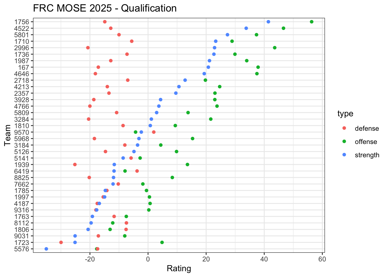
10.2.3 Offense-defense
Rather than only using the margin of victory (or the win/tie/loss result) we can also estimate offense and defense contribution of the players by utilizing both home and away scores.
Let \(S^H_g\) (\(S^A_g\)) be the points scored by the home team while a combination of players are on the court. Assume \[S^H_g = \sum_{p \in H[g]} \theta_p - \sum_{p\in A[g]} \delta_p + \epsilon^H_g\] and \[S^A_g = \sum_{p \in A[g]} \theta_p - \sum_{p\in H[g]} \delta_p+ \epsilon^A_g\]
We have the following parameters
\(\theta_p\) is the offensive rating of player \(p\) and
\(\delta_p\) is the defensive rating of player \(p\).
In this model, we only observe noisy estimates of the difference between offense and defense ratings. Thus we have an identifiability issue that will manifest itself in one of the estimates not being estimable. We will treat this non-estimable rating as 0 and we are allowed to add a constant to the \(\theta\)s and (the same constant) to the \(\delta\)s.
The parameters are transitive and thus the model is not capable of estimating complementary play among players on a team or match ups with opposing players.
If we assume \(\epsilon^H_g,\epsilon^A_g \stackrel{ind}{\sim} N(0,\sigma^2)\), then we have a regression model. To estimate the parameters in this regression model, we will need to construct two matrices that each have a row for each combination of players and a column for each player. In the home matrix, each cell is a 1 if that home player is in the combination and a 0 otherwise. In the home matrix, each cell is a 1 if that away player is in the combination and a 0 otherwise.
The margin of victory (and win-tie-loss) matrix is actually just the difference between the home and away matrix just described.
10.3 Examples
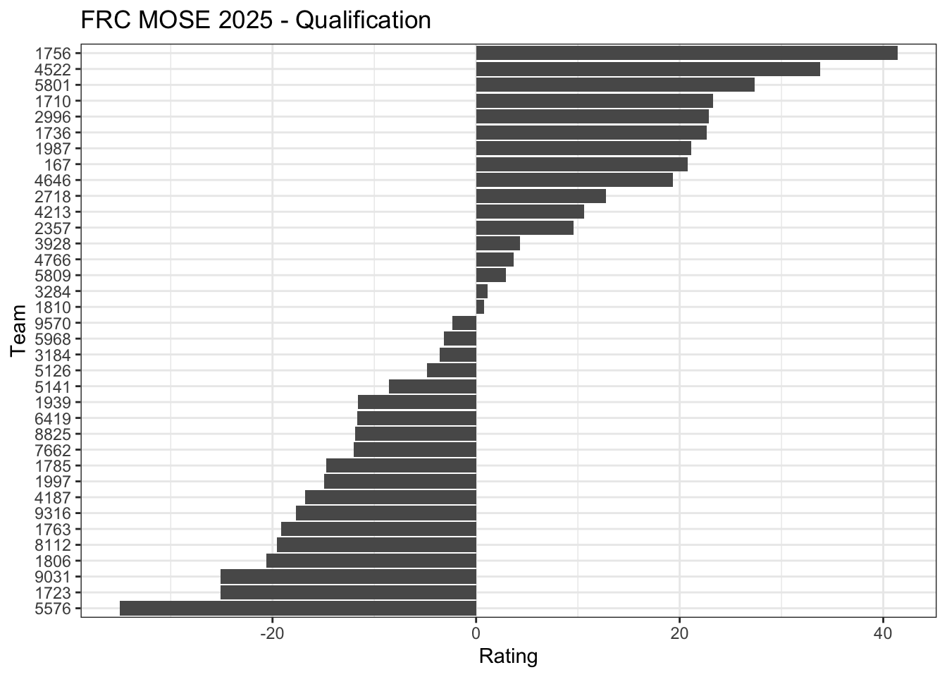
10.3.1 FRC MOSE 2025
The First Robotics Competition (FRC) is a high school robotics competition. Each match in an FRC competition pits two alliances (red and blue) each composed of 3 robots from different teams. The robots within an alliance cooperate and compete against the robots in the other alliance to score points. The alliance with more points at the end wins the match.
tmp <-read_csv("../../data/frc_mose2025.csv")
Rows: 66 Columns: 10
── Column specification ────────────────────────────────────────────────────────
Delimiter: ","
chr (2): Match, Start Time
dbl (8): Red 1, Red 2, Red 3, Blue 1, Blue 2, Blue 3, Red Final, Blue Final

ℹ Use `spec()` to retrieve the full column specification for this data.
ℹ Specify the column types or set `show_col_types = FALSE` to quiet this message.
# Construct model matricesX_red <-construct_matrix(mose2025, "Red 1", 36) +construct_matrix(mose2025, "Red 2", 36) +construct_matrix(mose2025, "Red 3", 36) X_blue <-construct_matrix(mose2025, "Blue 1", 36) +construct_matrix(mose2025, "Blue 2", 36) +construct_matrix(mose2025, "Blue 3", 36) # Team 8112 did not arrive on time and thus is missing in its first two matchestable(rowSums(X_red))
These models could be extended or modified in many different directions.
10.5.1 Time
In the FRC example, the time is fixed by the match duration. In other sports, the time may be variable as we are looking at how long a combination of players is on the field. Incorporating the duration on the field would have two impacts: 1) the expected margin (or scores) would be expected to increase and 2) the variability would increase.
If \(T_g\) is the time associated with margin \(M_g\), then we can modify our margin of victory model accordingly
Now, we need each row in our model matrix to be multiplied by the corresponding \(T_g\), e.g. multiply row 1 by \(T_1\). Then we can use weighted regression to incorporate \(T_g\) into the variance.
Our offense-defense contribution would be modified by
\[S^H_g = T_g\left(\sum_{p \in H[g]} \theta_p - \sum_{p\in A[g]} \delta_p \right)+ \epsilon^H_g,
\quad \epsilon^H_g \stackrel{ind}{\sim} N(0,T_g\sigma^2)\] and \[S^A_g = T_g\left(\sum_{p \in A[g]} \theta_p - \sum_{p\in H[g]} \delta_p \right)+ \epsilon^A_g,
\quad \epsilon^A_g \stackrel{ind}{\sim} N(0,T_g\sigma^2).\] To incorporate these changes, we would multiply each row in our matrices by the corresponding \(T_g\) and use weighted regression for the \(T_g\) in the variance.
10.5.2 Home advantage
The presentation here as ignored the home advantage. If we want to incorporate the home advantage (and we also have time) then we could add the home advantage into our model. In the margin of victory model \[M_g = T_g\left(\eta + \sum_{p \in H[g]} \theta_p - \sum_{p\in A[g]} \theta_p \right)+ \epsilon_g,
\quad \epsilon_g \stackrel{ind}{\sim} N(0,T_g \sigma^2).\] The interpretation of \(\eta\) would be per unit time using whatever time units were used for \(T_g\). To get the entire home advantage, we would calculate \(\eta \sum_{g=1}^G T_g\). A similar change can be made in the offense-defense model for \(S^H_g\).
10.5.3 Probability
Probability calculations in these models is performed similarly to probability calculations in the associated margin of victory, win-(tie)-loss, or offense-defense models. Since in these models we are looking at the contribution of players, for the probability calculation we will need to determine which combination of players we are looking at. Once we have determined those players, we will calculate the appropriate difference in ratings.
10.5.4 Small counts
I have previously mentioned that in sports with small counts, e.g. soccer or hockey, it may be preferable to utilize a win-(tie-)loss model. Even in high scoring sports, e.g. basketball, when we are looking at a specific combination of players on the court, then we may have a small number of points scored (for both sides) when that specific combination is on the court. Thus, we may want to look into use Poisson (or negative binomial) based models for the offense-defense rating.
A Poisson model may look something like
\[S^H_g \stackrel{ind}{\sim} Po(\lambda^H_g)\] with \[\log(\lambda^H_g) = \sum_{p \in H[g]} \theta_p - \sum_{p\in A[g]} \delta_p.\] In these models, the interpretation of the parameters changed are are mostly easily understood as their multiplicative effect. For example, \[E[S^H_g] = \left. \prod_{p \in H[g]} e^{\theta_p} \right/ \prod_{p \in A[g]} e^{\theta_p}.\]
10.5.5 Estimability
Recall that identifiability is based on whether the parameters can be estimated with any data, i.e. the best data, while estimability is based on whether parameters can be estimated with a particular data set. Player contributions in some sports are very difficult to estimate with these models because insufficient combinations of players are available. Baseball and softball generally have the same set of players playing the field and the battling order is the same. Soccer generally has the same set of players on the field, and the sport is low scoring. Volleyball generally has the same players in the same order on the court. Even a sport like basketball can be affected by this issue if one player is immediately subbed in or out when another player is subbed (either on the same team or the other team).